Parallel machine learning benchmarks
I recently wrote about New parallel computing frameworks in R. The goal of this blog is to explore how these new frameworks may be used for parallelizing machine learning benchmark experiments.
Introduction to machine learning
Typically when we parallelize machine learning benchmark experiments with mlr3, we use the following pipeline:
mlr3::benchmark_grid()creates a grid of tasks, learners, and resampling iterations.batchtools::makeExperimentRegistry()creates a registry directory.mlr3batchmark::batchmark()save the grid into the registry directory.batchtools::submitJobs()launches the jobs on the cluster.mlr3batchmark::reduceResultsBatchmark()combines the results into a single file.
This approach is discussed in the following blogs:
- The importance of hyper-parameter tuning explains how to use the auto-tuner.
- Cross-validation experiments with torch
learners explains
how to compare linear models in torch with other learners from
outside torch like
glmnet. - Torch learning with binary classification explains how to implement a custom loss function for binary classification in mlr3torch.
- Comparing neural network architectures using mlr3torch explains how to implement different neural network architectures, and make figures to compare their subtrain/validation/test error rates.
While this approach is very useful, there are some dis-advantages:
- jobs can have very different times, which induces an inefficient use of the scheduler (which requires specifying a single max time/memory for all heterogeneous tasks within a single job/experiment).
- the data must be serialized to the network file system, which can be slow.
Simulate data for ML experiment
This example is taken from ?mlr3resampling::pvalue:
N <- 80
library(data.table)
set.seed(1)
reg.dt <- data.table(
  x=runif(N, -2, 2),
  person=factor(rep(c("Alice","Bob"), each=0.5*N)))
reg.pattern.list <- list(
  easy=function(x, person)x^2,
  impossible=function(x, person)(x^2)*(-1)^as.integer(person))
SOAK <- mlr3resampling::ResamplingSameOtherSizesCV$new()
viz.dt.list <- list()
reg.task.list <- list()
for(pattern in names(reg.pattern.list)){
  f <- reg.pattern.list[[pattern]]
  task.dt <- data.table(reg.dt)[
  , y := f(x,person)+rnorm(N, sd=0.5)
  ][]
  task.obj <- mlr3::TaskRegr$new(
    pattern, task.dt, target="y")
  task.obj$col_roles$feature <- "x"
  task.obj$col_roles$stratum <- "person"
  task.obj$col_roles$subset <- "person"
  reg.task.list[[pattern]] <- task.obj
  viz.dt.list[[pattern]] <- data.table(pattern, task.dt)
}
(viz.dt <- rbindlist(viz.dt.list))
##         pattern          x person          y
##          <char>      <num> <fctr>      <num>
##   1:       easy -0.9379653  Alice  0.7975172
##   2:       easy -0.5115044  Alice  0.1349559
##   3:       easy  0.2914135  Alice  0.4334035
##   4:       easy  1.6328312  Alice  2.9444692
##   5:       easy -1.1932723  Alice  1.0795209
##  ---
## 156: impossible  1.5687933    Bob  1.9371203
## 157: impossible  1.4573579    Bob  2.8444709
## 158: impossible -0.4400418    Bob -0.3142869
## 159: impossible  1.1092828    Bob  1.4364957
## 160: impossible  1.8424720    Bob  3.2041650
The data table above represents simulated regression problem, which is visualized using the code below.
library(ggplot2)
ggplot()+
  geom_point(aes(
    x, y),
    data=viz.dt)+
  facet_grid(pattern ~ person, labeller=label_both)
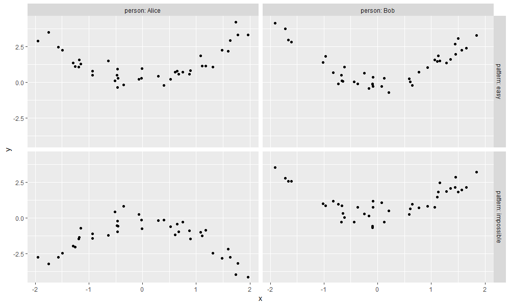
The figure above shows data for two simulated patterns:
- easy (top) has same pattern in the two people.
- impossible (bottom) has different patterns in the two people.
mlr3 benchmark grid
To use mlr3 on these data, we create a benchmark grid with a list of tasks and learners in the code below.
reg.learner.list <- list(
  mlr3::LearnerRegrFeatureless$new())
if(requireNamespace("rpart")){
  reg.learner.list$rpart <- mlr3::LearnerRegrRpart$new()
}
(bench.grid <- mlr3::benchmark_grid(
  reg.task.list,
  reg.learner.list,
  SOAK))
##          task          learner          resampling
##        <char>           <char>              <char>
## 1:       easy regr.featureless same_other_sizes_cv
## 2:       easy       regr.rpart same_other_sizes_cv
## 3: impossible regr.featureless same_other_sizes_cv
## 4: impossible       regr.rpart same_other_sizes_cv
The output above indicates that we want to run same_other_sizes_cv
resampling on two different tasks, and two different learners.
To run that in sequence, we use the typical mlr3 functions in the code below.
bench.result <- mlr3::benchmark(bench.grid)
bench.score <- mlr3resampling::score(bench.result, mlr3::msr("regr.rmse"))
bench.score[, .(task_id, algorithm, train.subsets, test.fold, test.subset, regr.rmse)]
##        task_id   algorithm train.subsets test.fold test.subset regr.rmse
##         <char>      <char>        <char>     <int>      <fctr>     <num>
##  1:       easy featureless           all         1       Alice 0.8417981
##  2:       easy featureless           all         1         Bob 1.4748311
##  3:       easy featureless           all         2       Alice 1.3892457
##  4:       easy featureless           all         2         Bob 1.2916491
##  5:       easy featureless           all         3       Alice 1.1636785
##  6:       easy featureless           all         3         Bob 1.0491199
##  7:       easy featureless         other         1       Alice 0.8559209
##  8:       easy featureless         other         1         Bob 1.4567103
##  9:       easy featureless         other         2       Alice 1.3736439
## 10:       easy featureless         other         2         Bob 1.2943787
## 11:       easy featureless         other         3       Alice 1.1395756
## 12:       easy featureless         other         3         Bob 1.0899069
## 13:       easy featureless          same         1       Alice 0.8667528
## 14:       easy featureless          same         1         Bob 1.5148801
## 15:       easy featureless          same         2       Alice 1.4054366
## 16:       easy featureless          same         2         Bob 1.2897447
## 17:       easy featureless          same         3       Alice 1.1917033
## 18:       easy featureless          same         3         Bob 1.0118805
## 19:       easy       rpart           all         1       Alice 0.6483484
## 20:       easy       rpart           all         1         Bob 0.5780414
## 21:       easy       rpart           all         2       Alice 0.7737929
## 22:       easy       rpart           all         2         Bob 0.6693803
## 23:       easy       rpart           all         3       Alice 0.4360203
## 24:       easy       rpart           all         3         Bob 0.5599774
## 25:       easy       rpart         other         1       Alice 0.7000487
## 26:       easy       rpart         other         1         Bob 1.3295572
## 27:       easy       rpart         other         2       Alice 1.2688572
## 28:       easy       rpart         other         2         Bob 0.9847977
## 29:       easy       rpart         other         3       Alice 0.8686188
## 30:       easy       rpart         other         3         Bob 0.8957394
## 31:       easy       rpart          same         1       Alice 0.9762360
## 32:       easy       rpart          same         1         Bob 1.3404500
## 33:       easy       rpart          same         2       Alice 1.1213335
## 34:       easy       rpart          same         2         Bob 1.1853491
## 35:       easy       rpart          same         3       Alice 0.7931738
## 36:       easy       rpart          same         3         Bob 0.9980859
## 37: impossible featureless           all         1       Alice 1.8015752
## 38: impossible featureless           all         1         Bob 2.0459690
## 39: impossible featureless           all         2       Alice 1.9332069
## 40: impossible featureless           all         2         Bob 1.3513960
## 41: impossible featureless           all         3       Alice 1.4087384
## 42: impossible featureless           all         3         Bob 1.5117399
## 43: impossible featureless         other         1       Alice 2.7435334
## 44: impossible featureless         other         1         Bob 3.0650008
## 45: impossible featureless         other         2       Alice 3.0673372
## 46: impossible featureless         other         2         Bob 2.4200628
## 47: impossible featureless         other         3       Alice 2.5631614
## 48: impossible featureless         other         3         Bob 2.7134959
## 49: impossible featureless          same         1       Alice 1.1982239
## 50: impossible featureless          same         1         Bob 1.2037929
## 51: impossible featureless          same         2       Alice 1.2865945
## 52: impossible featureless          same         2         Bob 1.1769211
## 53: impossible featureless          same         3       Alice 1.0677617
## 54: impossible featureless          same         3         Bob 0.9738987
## 55: impossible       rpart           all         1       Alice 1.9942054
## 56: impossible       rpart           all         1         Bob 2.9047858
## 57: impossible       rpart           all         2       Alice 1.9339810
## 58: impossible       rpart           all         2         Bob 1.6467536
## 59: impossible       rpart           all         3       Alice 1.6622025
## 60: impossible       rpart           all         3         Bob 1.7632037
## 61: impossible       rpart         other         1       Alice 2.9498727
## 62: impossible       rpart         other         1         Bob 3.0738533
## 63: impossible       rpart         other         2       Alice 3.5994187
## 64: impossible       rpart         other         2         Bob 2.9526543
## 65: impossible       rpart         other         3       Alice 2.5892647
## 66: impossible       rpart         other         3         Bob 3.1410587
## 67: impossible       rpart          same         1       Alice 0.9056522
## 68: impossible       rpart          same         1         Bob 1.3881235
## 69: impossible       rpart          same         2       Alice 0.8927662
## 70: impossible       rpart          same         2         Bob 0.7149474
## 71: impossible       rpart          same         3       Alice 0.9229746
## 72: impossible       rpart          same         3         Bob 0.6295206
##        task_id   algorithm train.subsets test.fold test.subset regr.rmse
##         <char>      <char>        <char>     <int>      <fctr>     <num>
The table of scores above shows the root mean squared error for each combination of task, algorithm, train subset, test fold, and test subset. These error values are summarized in the visualization below.
bench.plist <- mlr3resampling::pvalue(bench.score)
plot(bench.plist)
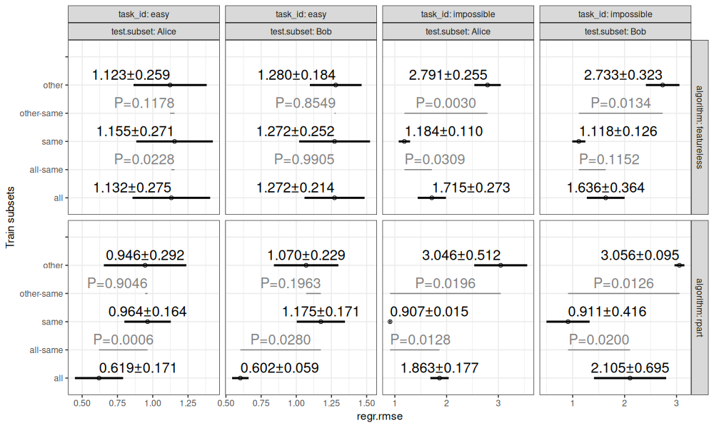
The figure above shows:
- in black, mean plus or minus standard deviation, for each combination of task, test subset, algorithm, and train subsets.
- in grey, P-values for differences between same/all and same/other (two-sided paired T-test).
Porting to targets
To run the same computations using targets, we first loop over the benchmark grid, and create a data table with one row per train/test split.
target_dt_list <- list()
for(bench_row in seq_along(bench.grid$resampling)){
  cv <- bench.grid$resampling[[bench_row]]
  cv$instantiate(bench.grid$task[[bench_row]])
  it_vec <- seq_len(cv$iters)
  target_dt_list[[bench_row]] <- data.table(bench_row, iteration=it_vec)
}
(target_dt <- rbindlist(target_dt_list))
##     bench_row iteration
##         <int>     <int>
##  1:         1         1
##  2:         1         2
##  3:         1         3
##  4:         1         4
##  5:         1         5
##  6:         1         6
##  7:         1         7
##  8:         1         8
##  9:         1         9
## 10:         1        10
## 11:         1        11
## 12:         1        12
## 13:         1        13
## 14:         1        14
## 15:         1        15
## 16:         1        16
## 17:         1        17
## 18:         1        18
## 19:         2         1
## 20:         2         2
## 21:         2         3
## 22:         2         4
## 23:         2         5
## 24:         2         6
## 25:         2         7
## 26:         2         8
## 27:         2         9
## 28:         2        10
## 29:         2        11
## 30:         2        12
## 31:         2        13
## 32:         2        14
## 33:         2        15
## 34:         2        16
## 35:         2        17
## 36:         2        18
## 37:         3         1
## 38:         3         2
## 39:         3         3
## 40:         3         4
## 41:         3         5
## 42:         3         6
## 43:         3         7
## 44:         3         8
## 45:         3         9
## 46:         3        10
## 47:         3        11
## 48:         3        12
## 49:         3        13
## 50:         3        14
## 51:         3        15
## 52:         3        16
## 53:         3        17
## 54:         3        18
## 55:         4         1
## 56:         4         2
## 57:         4         3
## 58:         4         4
## 59:         4         5
## 60:         4         6
## 61:         4         7
## 62:         4         8
## 63:         4         9
## 64:         4        10
## 65:         4        11
## 66:         4        12
## 67:         4        13
## 68:         4        14
## 69:         4        15
## 70:         4        16
## 71:         4        17
## 72:         4        18
##     bench_row iteration
##         <int>     <int>
In the output above, bench_row is the row number of the benchmark
grid table, and iteration is the row number in the corresponding
instantiated resampling. To use these data with targets, we first
define a compute function.
compute <- function(target_num){
  ##library(data.table)
  target_row <- target_dt[target_num]
  it.dt <- bench.grid$resampling[[target_row$bench_row]]$instance$iteration.dt
  L <- bench.grid$learner[[target_row$bench_row]]
  this_task <- bench.grid$task[[target_row$bench_row]]
  set_rows <- function(set_name)it.dt[[set_name]][[target_row$iteration]]
  L$train(this_task, set_rows("train"))
  pred <- L$predict(this_task, set_rows("test"))
  it.dt[target_row$iteration, .(
    task_id=this_task$id, algorithm=sub("regr.","",L$id),
    train.subsets, test.fold, test.subset,
    ##groups, seed, n.train.groups,
    regr.rmse=pred$score(mlr3::msrs("regr.rmse")))]
}
compute(1)
##    task_id   algorithm train.subsets test.fold test.subset regr.rmse
##     <char>      <char>        <char>     <int>      <fctr>     <num>
## 1:    easy featureless           all         1       Alice 0.9907855
compute(2)
##    task_id   algorithm train.subsets test.fold test.subset regr.rmse
##     <char>      <char>        <char>     <int>      <fctr>     <num>
## 1:    easy featureless           all         1         Bob  1.300868
We then save the data and function to a file on disk.
save(target_dt, bench.grid, compute, file="2025-05-20-mlr3-targets-in.RData")
Then we create a tar script which begins by reading the data, and ends with a list of targets.
targets::tar_script({
  load("2025-05-20-mlr3-targets-in.RData")
  job_targs <- tarchetypes::tar_map(
    list(target_num=seq_len(nrow(target_dt))),
    targets::tar_target(result, compute(target_num)))
  list(
    tarchetypes::tar_combine(combine, job_targs, command=rbind(!!!.x)),
    job_targs)
}, ask=FALSE)
The trick in the code above is the use of two functions:
tar_map()creates a target for each value oftarget_num, saving the list of targets tojob_targs.tar_combine()creates a target that depends on all of the targets in thejob_targslist.
The code below computes the results.
if(FALSE){
  targets::tar_manifest()
  targets::tar_visnetwork()
}
targets::tar_make()
## Error:
## ! Error in tar_make():
##   there is no package called 'tarchetypes'
##   See https://books.ropensci.org/targets/debugging.html
(tar_score_dt <- targets::tar_read(combine))
## Error:
## ! targets data store _targets not found. Utility functions like tar_read() and tar_load() require a pre-existing targets data store (default: _targets/) created by tar_make(), tar_make_clustermq(), or tar_make_future(). Details: https://books.ropensci.org/targets/data.html
The table above shows the test error, and the code below plots it.
tar_pval_list <- mlr3resampling::pvalue(tar_score_dt)
## Error: object 'tar_score_dt' not found
plot(tar_pval_list)
## Error: object 'tar_pval_list' not found
The result figure above is consistent with the result figure that was computed with the usual mlr3 benchmark function.
Dynamic targets
Next, we implement dynamic branching, which is apparently faster for lots of branches.
targets::tar_script({
  load("2025-05-20-mlr3-targets-in.RData")
  list(
    targets::tar_target(target_num, seq_len(nrow(target_dt))),
    targets::tar_target(result, compute(target_num), pattern=map(target_num)))
}, ask=FALSE)
The code above uses map(target_num) to create a different result for
each value of target_num, which is combined together into a single
result table, computed and shown below.
targets::tar_make()
## + target_num dispatched

## ✔ target_num completed [0ms, 99 B]

## + result declared [72 branches]

## ✔ result completed [1.7s, 20.34 kB]

## ✔ ended pipeline [3.1s, 73 completed, 0 skipped]
(dyn_score_dt <- targets::tar_read(result))
##        task_id   algorithm train.subsets test.fold test.subset regr.rmse
##         <char>      <char>        <char>     <int>      <fctr>     <num>
##  1:       easy featureless           all         1       Alice 0.9907855
##  2:       easy featureless           all         1         Bob 1.3008678
##  3:       easy featureless           all         2       Alice 0.9543573
##  4:       easy featureless           all         2         Bob 1.3303316
##  5:       easy featureless           all         3       Alice 1.3635807
##  6:       easy featureless           all         3         Bob 1.2370617
##  7:       easy featureless         other         1       Alice 0.9914137
##  8:       easy featureless         other         1         Bob 1.2762933
##  9:       easy featureless         other         2       Alice 0.9832029
## 10:       easy featureless         other         2         Bob 1.3212197
## 11:       easy featureless         other         3       Alice 1.3653704
## 12:       easy featureless         other         3         Bob 1.2055645
## 13:       easy featureless          same         1       Alice 1.0329491
## 14:       easy featureless          same         1         Bob 1.3572628
## 15:       easy featureless          same         2       Alice 0.9302700
## 16:       easy featureless          same         2         Bob 1.3432935
## 17:       easy featureless          same         3       Alice 1.3642008
## 18:       easy featureless          same         3         Bob 1.2703672
## 19:       easy       rpart           all         1       Alice 0.4311639
## 20:       easy       rpart           all         1         Bob 0.6687888
## 21:       easy       rpart           all         2       Alice 0.8491932
## 22:       easy       rpart           all         2         Bob 0.5917313
## 23:       easy       rpart           all         3       Alice 0.5898475
## 24:       easy       rpart           all         3         Bob 0.4972741
## 25:       easy       rpart         other         1       Alice 0.8816927
## 26:       easy       rpart         other         1         Bob 1.0974634
## 27:       easy       rpart         other         2       Alice 0.8300939
## 28:       easy       rpart         other         2         Bob 0.9037082
## 29:       easy       rpart         other         3       Alice 1.1442886
## 30:       easy       rpart         other         3         Bob 0.6604022
## 31:       easy       rpart          same         1       Alice 0.8544508
## 32:       easy       rpart          same         1         Bob 1.1207956
## 33:       easy       rpart          same         2       Alice 0.6105662
## 34:       easy       rpart          same         2         Bob 1.3054000
## 35:       easy       rpart          same         3       Alice 0.9651013
## 36:       easy       rpart          same         3         Bob 1.0334799
## 37: impossible featureless           all         1       Alice 1.9454542
## 38: impossible featureless           all         1         Bob 2.1334055
## 39: impossible featureless           all         2       Alice 1.7045394
## 40: impossible featureless           all         2         Bob 1.1520164
## 41: impossible featureless           all         3       Alice 1.4892815
## 42: impossible featureless           all         3         Bob 1.5684921
## 43: impossible featureless         other         1       Alice 2.7995421
## 44: impossible featureless         other         1         Bob 3.1692606
## 45: impossible featureless         other         2       Alice 2.9193144
## 46: impossible featureless         other         2         Bob 2.3225307
## 47: impossible featureless         other         3       Alice 2.6808761
## 48: impossible featureless         other         3         Bob 2.6837346
## 49: impossible featureless          same         1       Alice 1.5196359
## 50: impossible featureless          same         1         Bob 1.2789725
## 51: impossible featureless          same         2       Alice 0.9755388
## 52: impossible featureless          same         2         Bob 0.9608841
## 53: impossible featureless          same         3       Alice 0.8906583
## 54: impossible featureless          same         3         Bob 1.1235452
## 55: impossible       rpart           all         1       Alice 1.6741137
## 56: impossible       rpart           all         1         Bob 2.3836980
## 57: impossible       rpart           all         2       Alice 1.8404374
## 58: impossible       rpart           all         2         Bob 0.8826633
## 59: impossible       rpart           all         3       Alice 1.6903242
## 60: impossible       rpart           all         3         Bob 1.7301464
## 61: impossible       rpart         other         1       Alice 3.0262472
## 62: impossible       rpart         other         1         Bob 3.3728469
## 63: impossible       rpart         other         2       Alice 2.9450909
## 64: impossible       rpart         other         2         Bob 2.4264216
## 65: impossible       rpart         other         3       Alice 2.7310131
## 66: impossible       rpart         other         3         Bob 3.1240620
## 67: impossible       rpart          same         1       Alice 1.2828829
## 68: impossible       rpart          same         1         Bob 1.1630270
## 69: impossible       rpart          same         2       Alice 0.7275858
## 70: impossible       rpart          same         2         Bob 0.4470869
## 71: impossible       rpart          same         3       Alice 0.9512479
## 72: impossible       rpart          same         3         Bob 1.0282527
##        task_id   algorithm train.subsets test.fold test.subset regr.rmse
##         <char>      <char>        <char>     <int>      <fctr>     <num>
The table above shows the test error for each train/test split, which we can visualize via the code below.
dyn_pval_list <- mlr3resampling::pvalue(dyn_score_dt)
plot(dyn_pval_list)
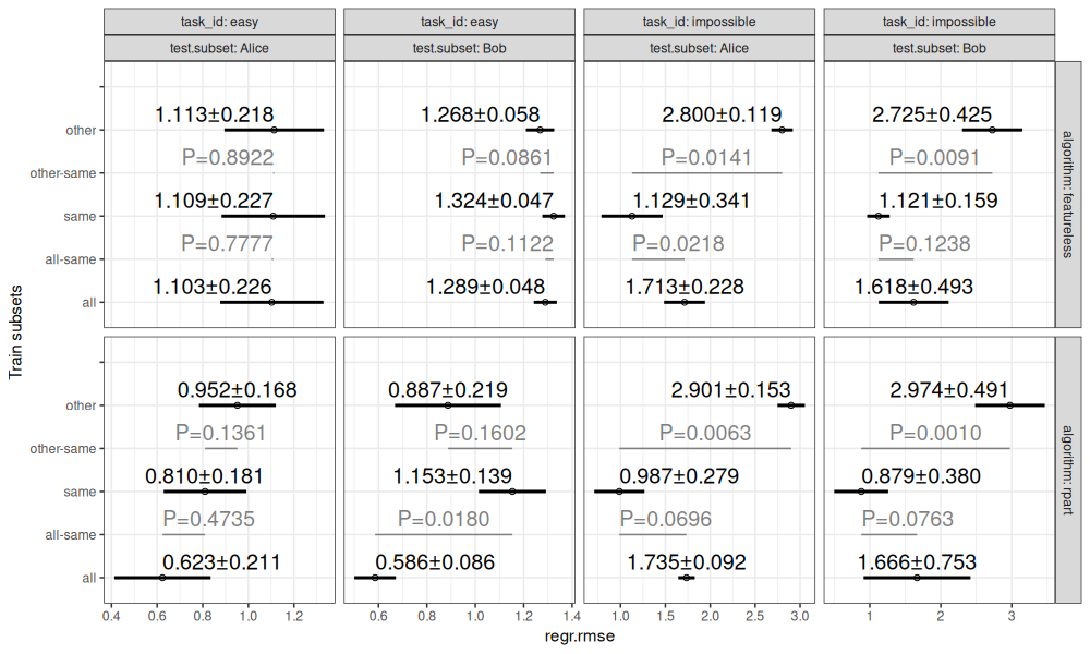
The graphics above are consistent with the previous result plots.
How does it work?
When you run tar_make(), files are created:
dir("_targets/objects/")
##  [1] "result_048013f7868011a2" "result_069f3e315217e27e" "result_06fbe6983d495e3e" "result_08182d7c2dd20ec3"
##  [5] "result_0a7ef7123d5dabba" "result_0ce4e0f358d155c2" "result_0cfba70ed70981ba" "result_112b8e8eb7cb2258"
##  [9] "result_19d8739f61397012" "result_1ad069a12018aded" "result_217edb41f1e1082c" "result_230c1adef6729d2a"
## [13] "result_2642222ace1a8999" "result_26eea39b7d448957" "result_30ad7aaf16e0425c" "result_3335271ef176ee7d"
## [17] "result_33fd60fe0ca79d55" "result_362cf35358864bd2" "result_374540b1e56f7c86" "result_3810136c1e7ea9dd"
## [21] "result_42c258fc60339ee0" "result_44073cf47ef7b79b" "result_4ce971cae9ec41b0" "result_4ea130c79d8b0145"
## [25] "result_505a84845a98b49f" "result_52403ac3c08f16b1" "result_5988fa8b2158f568" "result_629197c9dbf038d8"
## [29] "result_67a6334df4f3cb9f" "result_680cea198cec81c9" "result_6c441d6a6c30445c" "result_6f306d25112dfefc"
## [33] "result_782c1e65d42fbd5e" "result_7b9e20e914e1fb61" "result_816e13c2c98b9e18" "result_87f744b85f5dad72"
## [37] "result_89798851f17c5680" "result_93d076702b1a583c" "result_96d566b82b926d0d" "result_9923d497ceb6b102"
## [41] "result_9cf4fd39c387e4e3" "result_a0ff5af59f312179" "result_a32afd757f23673e" "result_a33abcbd8b6c98fe"
## [45] "result_a61ff9d7312ea260" "result_a68d3652aca4719a" "result_acfa949b32418563" "result_b374702926094bb2"
## [49] "result_b5e4139f56b67a58" "result_b742ae4f7df7cfde" "result_b919058f1fbddce3" "result_ba6896f8e7742065"
## [53] "result_bd433e7b7c989d62" "result_c02d2c95a677f106" "result_c3deea6fa5e4df56" "result_c5163c701caa8d22"
## [57] "result_c657ea0162b77a47" "result_c99aa5d7bf7eeae2" "result_cb00ccc443f5e8a0" "result_cc60dd0ed08ff3b4"
## [61] "result_ddb5f7dce171b8bc" "result_e4e1e52a9ba31254" "result_e5ce627ae4f143c5" "result_e67ea3f6d2a3af5a"
## [65] "result_e880aeaa6145c3a9" "result_f03929ed35b91f56" "result_f28570d89c20d11c" "result_f532d44d01f4b505"
## [69] "result_f8604114a575a8a2" "result_fba9b281047808f0" "result_fbe65e427b1c0cdb" "result_fd387e0d10c90edf"
## [73] "target_num"
Each target has a corresponding file.
How to run in parallel?
To run targets in parallel, you can use tar_option_set(controller=)
some crew controller, as explained on the Distributed computing
page. Below we use a
local crew of 2 workers.
unlink("_targets", recursive = TRUE)
targets::tar_script({
  tar_option_set(controller = crew::crew_controller_local(workers = 2))
  load("2025-05-20-mlr3-targets-in.RData")
  list(
    targets::tar_target(target_num, seq_len(nrow(target_dt))),
    targets::tar_target(result, compute(target_num), pattern=map(target_num)))
}, ask=FALSE)
targets::tar_make()
## + target_num dispatched

## ✔ target_num completed [0ms, 99 B]

## + result declared [72 branches]

## ✔ result completed [2.2s, 20.34 kB]

## ✔ ended pipeline [5.3s, 73 completed, 0 skipped]
targets::tar_read(result)
##        task_id   algorithm train.subsets test.fold test.subset regr.rmse
##         <char>      <char>        <char>     <int>      <fctr>     <num>
##  1:       easy featureless           all         1       Alice 0.9907855
##  2:       easy featureless           all         1         Bob 1.3008678
##  3:       easy featureless           all         2       Alice 0.9543573
##  4:       easy featureless           all         2         Bob 1.3303316
##  5:       easy featureless           all         3       Alice 1.3635807
##  6:       easy featureless           all         3         Bob 1.2370617
##  7:       easy featureless         other         1       Alice 0.9914137
##  8:       easy featureless         other         1         Bob 1.2762933
##  9:       easy featureless         other         2       Alice 0.9832029
## 10:       easy featureless         other         2         Bob 1.3212197
## 11:       easy featureless         other         3       Alice 1.3653704
## 12:       easy featureless         other         3         Bob 1.2055645
## 13:       easy featureless          same         1       Alice 1.0329491
## 14:       easy featureless          same         1         Bob 1.3572628
## 15:       easy featureless          same         2       Alice 0.9302700
## 16:       easy featureless          same         2         Bob 1.3432935
## 17:       easy featureless          same         3       Alice 1.3642008
## 18:       easy featureless          same         3         Bob 1.2703672
## 19:       easy       rpart           all         1       Alice 0.4311639
## 20:       easy       rpart           all         1         Bob 0.6687888
## 21:       easy       rpart           all         2       Alice 0.8491932
## 22:       easy       rpart           all         2         Bob 0.5917313
## 23:       easy       rpart           all         3       Alice 0.5898475
## 24:       easy       rpart           all         3         Bob 0.4972741
## 25:       easy       rpart         other         1       Alice 0.8816927
## 26:       easy       rpart         other         1         Bob 1.0974634
## 27:       easy       rpart         other         2       Alice 0.8300939
## 28:       easy       rpart         other         2         Bob 0.9037082
## 29:       easy       rpart         other         3       Alice 1.1442886
## 30:       easy       rpart         other         3         Bob 0.6604022
## 31:       easy       rpart          same         1       Alice 0.8544508
## 32:       easy       rpart          same         1         Bob 1.1207956
## 33:       easy       rpart          same         2       Alice 0.6105662
## 34:       easy       rpart          same         2         Bob 1.3054000
## 35:       easy       rpart          same         3       Alice 0.9651013
## 36:       easy       rpart          same         3         Bob 1.0334799
## 37: impossible featureless           all         1       Alice 1.9454542
## 38: impossible featureless           all         1         Bob 2.1334055
## 39: impossible featureless           all         2       Alice 1.7045394
## 40: impossible featureless           all         2         Bob 1.1520164
## 41: impossible featureless           all         3       Alice 1.4892815
## 42: impossible featureless           all         3         Bob 1.5684921
## 43: impossible featureless         other         1       Alice 2.7995421
## 44: impossible featureless         other         1         Bob 3.1692606
## 45: impossible featureless         other         2       Alice 2.9193144
## 46: impossible featureless         other         2         Bob 2.3225307
## 47: impossible featureless         other         3       Alice 2.6808761
## 48: impossible featureless         other         3         Bob 2.6837346
## 49: impossible featureless          same         1       Alice 1.5196359
## 50: impossible featureless          same         1         Bob 1.2789725
## 51: impossible featureless          same         2       Alice 0.9755388
## 52: impossible featureless          same         2         Bob 0.9608841
## 53: impossible featureless          same         3       Alice 0.8906583
## 54: impossible featureless          same         3         Bob 1.1235452
## 55: impossible       rpart           all         1       Alice 1.6741137
## 56: impossible       rpart           all         1         Bob 2.3836980
## 57: impossible       rpart           all         2       Alice 1.8404374
## 58: impossible       rpart           all         2         Bob 0.8826633
## 59: impossible       rpart           all         3       Alice 1.6903242
## 60: impossible       rpart           all         3         Bob 1.7301464
## 61: impossible       rpart         other         1       Alice 3.0262472
## 62: impossible       rpart         other         1         Bob 3.3728469
## 63: impossible       rpart         other         2       Alice 2.9450909
## 64: impossible       rpart         other         2         Bob 2.4264216
## 65: impossible       rpart         other         3       Alice 2.7310131
## 66: impossible       rpart         other         3         Bob 3.1240620
## 67: impossible       rpart          same         1       Alice 1.2828829
## 68: impossible       rpart          same         1         Bob 1.1630270
## 69: impossible       rpart          same         2       Alice 0.7275858
## 70: impossible       rpart          same         2         Bob 0.4470869
## 71: impossible       rpart          same         3       Alice 0.9512479
## 72: impossible       rpart          same         3         Bob 1.0282527
##        task_id   algorithm train.subsets test.fold test.subset regr.rmse
##         <char>      <char>        <char>     <int>      <fctr>     <num>
Above we see that the same result table has been computed in parallel.
Conclusions
We can use targets to declare and compute machine learning benchmark
experiments in parallel. Next steps will be to verify if this approach
works for larger experiments on the SLURM compute cluster, with
different sized data sets, and algorithms with different run-times.
Update: I tried it and got an error.
Session info
sessionInfo()
## R version 4.5.1 (2025-06-13 ucrt)
## Platform: x86_64-w64-mingw32/x64
## Running under: Windows 11 x64 (build 26100)
##
## Matrix products: default
##   LAPACK version 3.12.1
##
## locale:
## [1] LC_COLLATE=English_United States.utf8  LC_CTYPE=English_United States.utf8    LC_MONETARY=English_United States.utf8
## [4] LC_NUMERIC=C                           LC_TIME=English_United States.utf8
##
## time zone: America/Toronto
## tzcode source: internal
##
## attached base packages:
## [1] stats     graphics  utils     datasets  grDevices methods   base
##
## other attached packages:
## [1] mlr3resampling_2025.7.30 mlr3_1.1.0               future_1.67.0            ggplot2_3.5.2
## [5] data.table_1.17.99
##
## loaded via a namespace (and not attached):
##  [1] base64url_1.4        gtable_0.3.6         future.apply_1.20.0  dplyr_1.1.4          compiler_4.5.1
##  [6] crayon_1.5.3         rpart_4.1.24         tidyselect_1.2.1     parallel_4.5.1       callr_3.7.6
## [11] globals_0.18.0       scales_1.4.0         yaml_2.3.10          uuid_1.2-1           R6_2.6.1
## [16] labeling_0.4.3       generics_0.1.4       igraph_2.1.4         knitr_1.50           targets_1.11.3
## [21] palmerpenguins_0.1.1 backports_1.5.0      checkmate_2.3.3      tibble_3.3.0         paradox_1.0.1
## [26] pillar_1.11.0        RColorBrewer_1.1-3   mlr3measures_1.0.0   rlang_1.1.6          lgr_0.5.0
## [31] xfun_0.53            mlr3misc_0.18.0      cli_3.6.5            withr_3.0.2          magrittr_2.0.3
## [36] ps_1.9.1             processx_3.8.6       digest_0.6.37        grid_4.5.1           rstudioapi_0.17.1
## [41] secretbase_1.0.5     lifecycle_1.0.4      prettyunits_1.2.0    vctrs_0.6.5          evaluate_1.0.5
## [46] glue_1.8.0           farver_2.1.2         listenv_0.9.1        codetools_0.2-20     parallelly_1.45.1
## [51] tools_4.5.1          pkgconfig_2.0.3