The importance of hyper-parameter tuning
The goal of this blog post is to compare a machine learning algorithms, and demonstrate the importance of learning model complexity hyper-parameters, if the goal is to minimize prediction error (and that is always the goal in ML).
Theoretical discussion and visualizations
What is model complexity and why does it need to be controlled? Model complexity is the ability of a learning algorithm to fit complex patterns which are encoded in the train set. There is a different measure of model complexity for every learning algorithm:
- number of neighbors in K-nearest-neighbors,
- degree of L1 regularization in LASSO (as implemented in glmnet package in R),
- degree of polynomial in linear model basis expansion,
- cost parameter in support vector machines,
- number of iterations and learning rate in boosting (as implemented in xgboost package in R),
- number of gradient descent iterations (epochs), learning rate, number of hidden units, number of layers, etc, in neural networks.
In each machine learning algorithm, the model complexity must be controlled, by selecting a good value for the corresponding hyper-parameter. I created a data visualization which shows how this works using nearest neighbors (need to learn number of neighbors) and linear models (need to learn the degree of the polynomial basis expansion), for several regression problems.
- There are four different simulated data sets, each with a pattern of different complexity (constant, linear, quadratic, cubic).
- The linear model polynomial degree varies from 0 (constant prediction function, most regularized, least complex) to 9 (very wiggly prediction function that perfectly interpolates every train data point, least regularized, most complex).
- The number of neighbors varies from 1 (very wiggly prediction function that perfectly interpolates every train data point, least regularized, most complex) to 10 (constant prediction function, most regularized, least complex).
- These two learning algorithms are interesting examples to compare, because the least complex model (in both cases) always predicts the average of the train labels. That turns out to be the best prediction function, in the case of the constant data/pattern.
- But for the other data/patterns, a more complex regularization parameter must be used to get optimal prediction accuracy. For example, the regularization parameters which gives minimal test error for the linear data/pattern are 3 nearest neighbors, and polynomial degree 1.
The goal of this blog is to demonstrate how to use mlr3 auto tuner to properly learn such hyper-parameters, and show that approach is more accurate than using the defaults (which may be ok for some data, but sub-optimal for others).
Simulation
Below we define some simulated data, for five different regression problems, of varying complexity.
max.x <- 12
min.x <- -max.x
fun.list <- list(
  constant=function(x)1,
  linear=function(x)x/3,
  quadratic=function(x)x^2/max.x-5,
  sin=function(x)4*sin(x),
  step=function(x)ifelse(x<0, 4, -4))
N <- 200
set.seed(1)
input.vec <- runif(N, min.x, max.x)
library(data.table)
task.list <- list()
sim.dt.list <- list()
for(fun.name in names(fun.list)){
  f <- fun.list[[fun.name]]
  true.vec <- f(input.vec)
  task.dt <- data.table(
    input=input.vec,
    output=true.vec+rnorm(N,sd=2))
  task.list[[fun.name]] <- mlr3::TaskRegr$new(
    fun.name, task.dt, target="output"
  )
  sim.dt.list[[fun.name]] <- data.table(fun.name, task.dt)
}
(sim.dt <- rbindlist(sim.dt.list))
##       fun.name     input     output
##         <char>     <num>      <num>
##    1: constant -5.627792 -0.2407334
##    2: constant -3.069026  1.0842317
##    3: constant  1.748481 -0.8218433
##    4: constant  9.796987  1.3160575
##    5: constant -7.159634 -0.3091693
##   ---
##  996:     step  2.173756 -8.1816922
##  997:     step -9.351345  7.3947878
##  998:     step  8.172169 -1.8722377
##  999:     step -4.368872  2.4667667
## 1000:     step  6.788432 -3.2359849
library(ggplot2)
ggplot()+
  geom_point(aes(
    input, output),
    data=sim.dt)+
  facet_grid(. ~ fun.name, labeller=label_both)
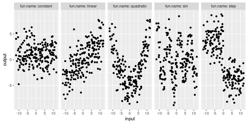
The plot above visualizes the simulated data. The goal of each learning algorithm is to learn the pattern in each of the five different data sets. To do that, we define a few different learning algorithms in the next section.
Learning algorithm definitions
Perhaps the simplest learning algorithm is nearest neighbors, which can be implemented in the mlr3 framework using the code below.
nn.default <- mlr3learners::LearnerRegrKKNN$new()
nn.default$param_set
## <ParamSet>
##             id    class lower upper nlevels default  value
##         <char>   <char> <num> <num>   <num>  <list> <list>
## 1:           k ParamInt     1   Inf     Inf       7      7
## 2:    distance ParamDbl     0   Inf     Inf       2
## 3:      kernel ParamFct    NA    NA      10 optimal
## 4:       scale ParamLgl    NA    NA       2    TRUE
## 5:     ykernel ParamUty    NA    NA     Inf
## 6: store_model ParamLgl    NA    NA       2   FALSE
The code above defines the default nearest neighbors regressor, which
has a default value of k=7 (that is the number of neighbors). As
discussed above, the number of neighbors is an important model
complexity hyper-parameter, which must be tuned for optimal prediction
accuracy. In other words, the default value 7 may provide sub-optimal
prediction accuracy, depending on the data set. Another option is to
manually select a different value for the number of neighbors, which
we do in the code below,
nn1 <- mlr3learners::LearnerRegrKKNN$new()
nn1$id <- "1 nearest neighbor"
nn1$param_set$values$k <- 1
The code above defines another nearest neighbor regressor, which uses 1 nearest neighbor, instead of the default 7. That may be better for some data sets, but in general, we would like to choose a different number of neighbors for each data set. We can do that using cross-validation, by dividing the train set into subtrain/validation sets, where the validation set is used to determine the optimal number of neighbors. The code below defines 5-fold cross-validation as the method to use,
subtrain.valid.cv <- mlr3::ResamplingCV$new()
subtrain.valid.cv$param_set$values$folds <- 5
Next, in the code below, we define a new nearest neighbor regressor, and tell mlr3 to tune the number of neighbors.
knn.learner <- mlr3learners::LearnerRegrKKNN$new()
knn.learner$param_set$values$k <- paradox::to_tune(1, 20)
To convert that to a learning algorithm that can be used in a
benchmark experiment, we need to use as the learner in an
auto_tuner, as in the code below,
knn.tuned = mlr3tuning::auto_tuner(
  tuner = mlr3tuning::TunerGridSearch$new(),
  learner = knn.learner,
  resampling = subtrain.valid.cv,
  measure = mlr3::msr("regr.mse"))
The code above says that we want to tune the learner using grid search, 5-fold CV, and select the model which minimizes MSE on the validation set.
Another non-linear regression algorithm is boosting, which can be
implemented in mlr3 using the code below. Again there are several
hyper-parameters which control model complexity, and in the code below
we tune two of them (eta=step size, nrounds=number of boosting
iterations). Note that some parameters should be tuned on the log
scale (like eta with log=TRUE in the code below), and others can be
tuned on the linear scale (like nrounds). Finally note in the code
below that we use a grid search with resolution 5 in order to save
time (default is 10 so with 2 hyper-parameters that would make 100
combinations, exercise for the reader to try that instead).
xgboost.learner <- mlr3learners::LearnerRegrXgboost$new()
xgboost.learner$param_set$values$eta <- paradox::to_tune(0.001, 1, log=TRUE)
xgboost.learner$param_set$values$nrounds <- paradox::to_tune(1, 100)
grid.search.5 <- mlr3tuning::TunerGridSearch$new()
grid.search.5$param_set$values$resolution <- 5
xgboost.tuned = mlr3tuning::auto_tuner(
  tuner = grid.search.5,
  learner = xgboost.learner,
  resampling = subtrain.valid.cv,
  measure = mlr3::msr("regr.mse"))
You might wonder about the code above, how did I know to tune eta from 0.001 to 1, and nrounds from 1 to 100? What are the good min/max values for each hyper-parameter? mlr3tuningspaces is a useful reference with data describing typical values for each hyper-parameter. And in fact, if you want to use the hyper-parameter ranges defined in that package, you can use code like below (ranger package for random forest).
ranger.tuned = mlr3tuning::auto_tuner(
  tuner = grid.search.5,
  learner = mlr3tuningspaces::lts(mlr3learners::LearnerRegrRanger$new()),
  resampling = subtrain.valid.cv,
  measure = mlr3::msr("regr.mse"))
Define benchmark experiment
After having defined the learning algorithms in the previous section, we combine them in the list below.
learner.list <- list(
  mlr3::LearnerRegrFeatureless$new(),
  mlr3learners::LearnerRegrRanger$new(), ranger.tuned,
  mlr3learners::LearnerRegrXgboost$new(), xgboost.tuned,
  knn.tuned, nn1, nn.default)
To see which of the learning algorithms is most accurate in each data set, we will use 3-fold cross-validation, as defined in ht code below.
train.test.cv <- mlr3::ResamplingCV$new()
train.test.cv$param_set$values$folds <- 3
In the code below, we define a benchmark grid, which combines tasks (data sets), with learners (algorithms), and resamplings (actually just one, 3-fold CV).
(bench.grid <- mlr3::benchmark_grid(
  tasks=task.list,
  learners=learner.list,
  resamplings=train.test.cv))
##          task            learner resampling
##        <char>             <char>     <char>
##  1:  constant   regr.featureless         cv
##  2:  constant        regr.ranger         cv
##  3:  constant  regr.ranger.tuned         cv
##  4:  constant       regr.xgboost         cv
##  5:  constant regr.xgboost.tuned         cv
##  6:  constant    regr.kknn.tuned         cv
##  7:  constant 1 nearest neighbor         cv
##  8:  constant          regr.kknn         cv
##  9:    linear   regr.featureless         cv
## 10:    linear        regr.ranger         cv
## 11:    linear  regr.ranger.tuned         cv
## 12:    linear       regr.xgboost         cv
## 13:    linear regr.xgboost.tuned         cv
## 14:    linear    regr.kknn.tuned         cv
## 15:    linear 1 nearest neighbor         cv
## 16:    linear          regr.kknn         cv
## 17: quadratic   regr.featureless         cv
## 18: quadratic        regr.ranger         cv
## 19: quadratic  regr.ranger.tuned         cv
## 20: quadratic       regr.xgboost         cv
## 21: quadratic regr.xgboost.tuned         cv
## 22: quadratic    regr.kknn.tuned         cv
## 23: quadratic 1 nearest neighbor         cv
## 24: quadratic          regr.kknn         cv
## 25:       sin   regr.featureless         cv
## 26:       sin        regr.ranger         cv
## 27:       sin  regr.ranger.tuned         cv
## 28:       sin       regr.xgboost         cv
## 29:       sin regr.xgboost.tuned         cv
## 30:       sin    regr.kknn.tuned         cv
## 31:       sin 1 nearest neighbor         cv
## 32:       sin          regr.kknn         cv
## 33:      step   regr.featureless         cv
## 34:      step        regr.ranger         cv
## 35:      step  regr.ranger.tuned         cv
## 36:      step       regr.xgboost         cv
## 37:      step regr.xgboost.tuned         cv
## 38:      step    regr.kknn.tuned         cv
## 39:      step 1 nearest neighbor         cv
## 40:      step          regr.kknn         cv
##          task            learner resampling
In the code below we tell the mlr3 logger to suppress most messages, then we run the benchmark experiment. Actually, if the results have already been computed and saved in the cache RData file, we just read that. Otherwise, you should run the code below that interactively, either on your own computer, or on a SLURM super-computer cluster. There are only 120 iterations in this case, but if you run that on a super-computer cluster, then it could potentially run 120x faster. It is better to use a super-computer for larger experiments, with more data sets, learning algorithms, and cross-validation folds. For example I have recently computed some machine learning experiments with over 1000 benchmark iterations, each of which can be computed in parallel (and very quickly using NAU Monsoon which has 4000 CPUs). See mlr3batchmark for computing these iterations in parallel using the batchtools R package (which supports backends such as SLURM, which is how things are parallelized on super-computers such as NAU Monsoon). See my R batchtools on Monsoon tutorial for more info.
lgr::get_logger("mlr3")$set_threshold("warn")
cache.RData <- "2024-01-29-hyper-parameter-tuning.RData"
if(file.exists(cache.RData)){
  load(cache.RData)
}else{#code below should be run interactively.
  if(on.cluster){
    reg.dir <- "2024-01-29-hyper-parameter-tuning-registry"
    unlink(reg.dir, recursive=TRUE)
    reg = batchtools::makeExperimentRegistry(
      file.dir = reg.dir,
      seed = 1,
      packages = "mlr3verse"
    )
    mlr3batchmark::batchmark(
      bench.grid, store_models = TRUE, reg=reg)
    job.table <- batchtools::getJobTable(reg=reg)
    chunks <- data.frame(job.table, chunk=1)
    batchtools::submitJobs(chunks, resources=list(
      walltime = 60*60,#seconds
      memory = 2000,#megabytes per cpu
      ncpus=1,  #>1 for multicore/parallel jobs.
      ntasks=1, #>1 for MPI jobs.
      chunks.as.arrayjobs=TRUE), reg=reg)
    batchtools::getStatus(reg=reg)
    jobs.after <- batchtools::getJobTable(reg=reg)
    table(jobs.after$error)
    ids <- jobs.after[is.na(error), job.id]
    bench.result <- mlr3batchmark::reduceResultsBatchmark(ids, reg = reg)
  }else{
    ## In the code below, we declare a multisession future plan to
    ## compute each benchmark iteration in parallel on this computer
    ## (data set, learning algorithm, cross-validation fold). For a
    ## few dozen iterations, using the multisession backend is
    ## probably sufficient (I have 12 CPUs on my work PC).
    if(require(future))plan("multisession")
    bench.result <- mlr3::benchmark(
      bench.grid, store_models = TRUE)
  }
  save(bench.result, file=cache.RData)
}
If you are following along, now is the time to grab a cup of tea or coffee.
Comparing tuned to default/fixed hyper-parameters
After having computed the benchmark result in the previous section, we use the score method below to compute a data table with columns for train time and mean squared test error.
bench.score <- bench.result$score(mlr3::msrs(c("time_train","regr.mse")))
bench.score[1]
##       nr  task_id       learner_id resampling_id iteration time_train regr.mse
##    <int>   <char>           <char>        <char>     <int>      <num>    <num>
## 1:     1 constant regr.featureless            cv         1       0.01 4.650449
## Hidden columns: uhash, task, learner, resampling, prediction
First, we create a new algorithm factor column in the code below, and take the subset of results for the nearest neighbors learning algorithms.
algo.levs <- c(
  "regr.ranger.tuned", "regr.ranger",
  "regr.xgboost.tuned", "regr.xgboost",
  "regr.kknn.tuned", nn.default$id, nn1$id,
  "regr.featureless")
only.nn <- bench.score[
, algorithm := factor(learner_id, algo.levs)
][
  grepl("nn|featureless|neighbor", algorithm)
]
We use the code below to visualize the nearest neighbors test error values.
ggplot()+
  geom_point(aes(
    regr.mse, algorithm),
    shape=1,
    data=only.nn)+
  facet_grid(. ~ task_id, labeller=label_both, scales="free")+
  scale_x_log10(
    "Mean squared prediction error on the test set")
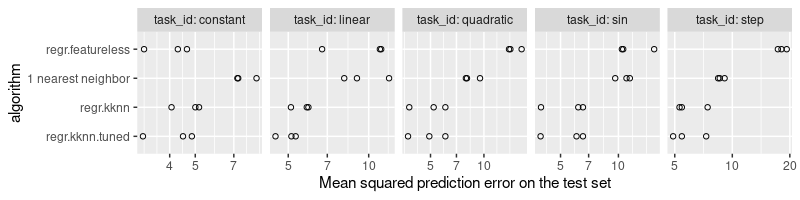
The plot above shows the mean squared prediction error on the X axis, and the learning algorithm on the Y axis. The three versions of nearest neighbors are shown, along with the baseline featureless predictor (which always predicts a constant value, the mean of the train labels). It is clear that
- the 1 nearest neighbor algorithm is the least accurate learning algorithm, and sometimes even has larger test error rates than the featureless baseline (in the constant and linear data).
- the regr.kknn algorithm (default/fixed number of neighbors is 7) yields reasonable predictions, which are most of the time better than the featureless baseline (except in the constant task).
- the regr.kknn.tuned algorithm has the least prediction error overall, because it uses an internal grid search to select the best number of neighbors, as a function of the training data.
The code below computes the selected number of neighbors for the tuned nearest neighbor algorithms:
only.nn[
  grepl("tuned", algorithm),
  data.table(
    task_id,
    neighbors=sapply(learner, function(L)L$tuning_result$k))
]
##       task_id neighbors
##        <char>     <int>
##  1:  constant        16
##  2:  constant        20
##  3:  constant        20
##  4:    linear        20
##  5:    linear        20
##  6:    linear        20
##  7: quadratic         9
##  8: quadratic         7
##  9: quadratic        12
## 10:       sin         9
## 11:       sin         9
## 12:       sin         7
## 13:      step        16
## 14:      step         7
## 15:      step        12
It is clear that the tuning procedure selected numbers of neighbors which are sometimes different from the fixed values we used in the other learners (1 and 7). As expected, we see larger number of neighbors for the simpler patterns (constant and linear).
Next, we examine the test error rates of the random forest learners.
only.ranger <- bench.score[grepl("featureless|ranger", algorithm)]
ggplot()+
  geom_point(aes(
    regr.mse, algorithm),
    shape=1,
    data=only.ranger)+
  facet_grid(. ~ task_id, labeller=label_both, scales="free")+
  scale_x_log10(
    "Mean squared prediction error on the test set")
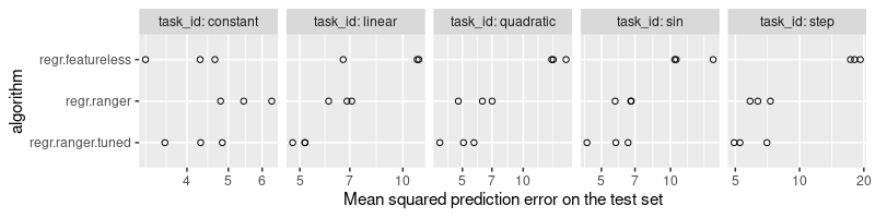
It is clear from the plot above that the tuned version is at least as accurate as the default, for each data set. In the case of the simpler tasks (constant and linear), the tuned version is substantially better.
Next, we examine the test error rates of the xgboost learners.
only.xgboost <- bench.score[grepl("xgboost|featureless", algorithm)]
ggplot()+
  geom_point(aes(
    regr.mse, algorithm),
    shape=1,
    data=only.xgboost)+
  facet_grid(. ~ task_id, labeller=label_both, scales="free")+
  scale_x_log10(
    "Mean squared prediction error on the test set")
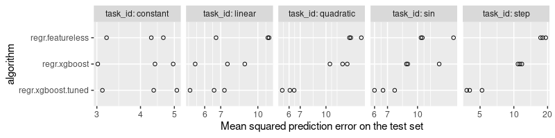
The plot above shows that the tuned learner is at least as accurate as the default, for each data set. The tuned learner has significantly smaller prediction error for the more complex patterns (quadratic, sin, step).
Comparing learning algorithms
In this section we compare the tuned versions of the learning algorithms with each other.
only.tuned <- bench.score[grepl("tuned|featureless", algorithm)]
ggplot()+
  geom_point(aes(
    regr.mse, algorithm),
    shape=1,
    data=only.tuned)+
  facet_grid(. ~ task_id, labeller=label_both, scales="free")+
  scale_x_log10(
    "Mean squared prediction error on the test set")
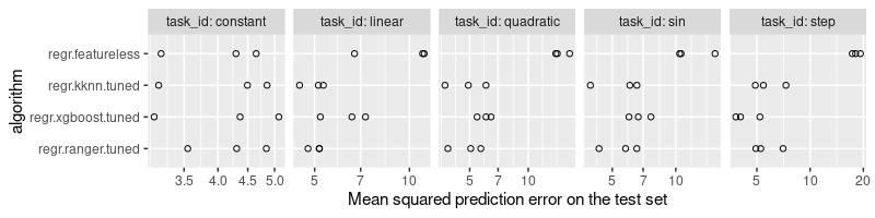
The plot above shows that there is no one algorithm that is the best for every data set, which is to be expected (no free lunch theorem). The best algorithm for task=step seems to be xgboost, whereas the nearest neighbors and ranger algorithms predict with similar optimality on the other non-trivial tasks (linear, quadratic, sin).
Comparing train time
In this section we compare the time it takes to train the algorithms.
ref <- function(seconds, unit){
  data.table(seconds, label=paste0("1 ", unit, " "))
}
ref.dt <- rbind(
  ref(60, "minute"),
  ref(1, "second"))
ggplot()+
  theme_bw()+
  geom_point(aes(
    time_train, algorithm),
    shape=1,
    data=bench.score)+
  geom_vline(aes(
    xintercept=seconds),
    color="grey",
    data=ref.dt)+
  geom_text(aes(
    seconds, Inf, label=label),
    color="grey50",
    data=ref.dt,
    angle=90,
    vjust=1.2,
    hjust=1)+
  facet_grid(. ~ task_id, labeller=label_both, scales="free")+
  scale_x_log10(
    "Training time (seconds)",
    breaks=10^seq(-2,2,by=2))
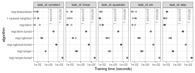
It is clear from the plot above that the hyper-parameter tuning takes significantly more time than the learning algorithms with default/fixed hyper-parameters. This is to be expected, because an internal grid search needs to be computed, in order to determine the optimal hyper-parameters for each train set. The increased computation time is the price you have to pay for the increased prediction accuracy.
Conclusions
We have explained how to implement hyper-parameter tuning, in the context of the mlr3 framework in R. We have shown that hyper-parameter tuning takes more time, but results in consistently more accurate predictions, with respect to learning algorithms which use default/fixed hyper-parameters. We have additionally showed how to implement mlr3 benchmark experiments on a SLURM cluster using mlr3batchmark/batchtools packages.
Session info
sessionInfo()
## R version 4.3.2 (2023-10-31)
## Platform: x86_64-pc-linux-gnu (64-bit)
## Running under: Ubuntu 22.04.3 LTS
##
## Matrix products: default
## BLAS:   /usr/lib/x86_64-linux-gnu/blas/libblas.so.3.10.0
## LAPACK: /usr/lib/x86_64-linux-gnu/lapack/liblapack.so.3.10.0
##
## locale:
##  [1] LC_CTYPE=fr_FR.UTF-8       LC_NUMERIC=C               LC_TIME=fr_FR.UTF-8        LC_COLLATE=fr_FR.UTF-8
##  [5] LC_MONETARY=fr_FR.UTF-8    LC_MESSAGES=fr_FR.UTF-8    LC_PAPER=fr_FR.UTF-8       LC_NAME=C
##  [9] LC_ADDRESS=C               LC_TELEPHONE=C             LC_MEASUREMENT=fr_FR.UTF-8 LC_IDENTIFICATION=C
##
## time zone: America/Phoenix
## tzcode source: system (glibc)
##
## attached base packages:
## [1] stats     graphics  utils     datasets  grDevices methods   base
##
## other attached packages:
## [1] future_1.33.1     ggplot2_3.4.4     data.table_1.15.0
##
## loaded via a namespace (and not attached):
##  [1] future.apply_1.11.1    gtable_0.3.4           highr_0.10             dplyr_1.1.4            compiler_4.3.2
##  [6] crayon_1.5.2           tidyselect_1.2.0       parallel_4.3.2         globals_0.16.2         scales_1.3.0
## [11] uuid_1.2-0             RhpcBLASctl_0.23-42    R6_2.5.1               mlr3tuning_0.19.2      labeling_0.4.3
## [16] generics_0.1.3         knitr_1.45.11          palmerpenguins_0.1.1   backports_1.4.1        checkmate_2.3.1
## [21] tibble_3.2.1           munsell_0.5.0          paradox_0.11.1         pillar_1.9.0           mlr3tuningspaces_0.4.0
## [26] mlr3measures_0.5.0     rlang_1.1.3            utf8_1.2.4             xfun_0.41.10           lgr_0.4.4
## [31] mlr3_0.17.2            mlr3misc_0.13.0        cli_3.6.2              withr_3.0.0            magrittr_2.0.3
## [36] digest_0.6.34          grid_4.3.2             mlr3learners_0.5.8     bbotk_0.7.3            lifecycle_1.0.4
## [41] vctrs_0.6.5            evaluate_0.23          glue_1.7.0             farver_2.1.1           listenv_0.9.1
## [46] codetools_0.2-19       parallelly_1.36.0      fansi_1.0.6            colorspace_2.1-0       tools_4.3.2
## [51] pkgconfig_2.0.3