Load-balanced parallel machine learning benchmarks
I recently wrote about Centralized vs de-centralized parallelization. The goal of this blog is to explore how these new frameworks may be used for parallelizing machine learning benchmark experiments.
Introduction to machine learning
Typically when we parallelize machine learning benchmark experiments with mlr3, we use the following pipeline:
mlr3::benchmark_grid()creates a grid of tasks, learners, and resampling iterations.batchtools::makeExperimentRegistry()creates a registry directory.mlr3batchmark::batchmark()save the grid into the registry directory.batchtools::submitJobs()launches the jobs on the cluster.mlr3batchmark::reduceResultsBatchmark()combines the results into a single file.
This approach is discussed in the following blogs:
- The importance of hyper-parameter tuning explains how to use the auto-tuner.
- Cross-validation experiments with torch
learners explains
how to compare linear models in torch with other learners from
outside torch like
glmnet. - Torch learning with binary classification explains how to implement a custom loss function for binary classification in mlr3torch.
- Comparing neural network architectures using mlr3torch explains how to implement different neural network architectures, and make figures to compare their subtrain/validation/test error rates.
While this approach is very useful, it assumes that submitJobs() can
efficiently run all the jobs in parallel, which is not always the case:
- Each ML job involves using a single learner on a single task, with a single train/test split.
- ML jobs can have very different times, which induces an inefficient use of the scheduler (which requires specifying a single max time/memory for all heterogeneous tasks within a single job/experiment).
- Some clusters like Alliance Canada allow a max of 1000 SLURM jobs per user at a time (or 1 SLURM job array with 1000 tasks). This includes all entries in the queue, which is problematic for some large-scale experiments. For example, our SOAK paper involved computing 1200+ jobs on the NAU Monsoon cluster, which did not impose the 1000 SLURM job limit.
In this blog, we investigate a method for overcoming this limitation:
- We create a certain number of SLURM jobs using batchtools.
- Each of these jobs looks for work to do in a central CSV table (one row per ML job), and saves the result to disk.
- A column in that table indicates state of job: not run yet, running, done.
- A lock file is used to ensure that only one SLURM job at a time can access and modify that table.
- When there are no more ML jobs with state “not run yet” then each worker process can exit.
First install dev mlr3resampling
Some code below requires a development version of mlr3resampling, so we install it first:
devtools::install_github("tdhock/mlr3resampling@proj")
## Using github PAT from envvar GITHUB_PAT. Use `gitcreds::gitcreds_set()` and unset GITHUB_PAT in .Renviron (or elsewhere) if you want to use the more secure git credential store instead.
## Skipping install of 'mlr3resampling' from a github remote, the SHA1 (c2220464) has not changed since last install.
##   Use `force = TRUE` to force installation
Simulate data for ML experiment
This example is taken from ?mlr3resampling::pvalue:
N <- 80
library(data.table)
set.seed(1)
reg.dt <- data.table(
  x=runif(N, -2, 2),
  person=factor(rep(c("Alice","Bob"), each=0.5*N)))
reg.pattern.list <- list(
  easy=function(x, person)x^2,
  impossible=function(x, person)(x^2)*(-1)^as.integer(person))
SOAK <- mlr3resampling::ResamplingSameOtherSizesCV$new()
viz.dt.list <- list()
reg.task.list <- list()
for(pattern in names(reg.pattern.list)){
  f <- reg.pattern.list[[pattern]]
  task.dt <- data.table(reg.dt)[
  , y := f(x,person)+rnorm(N, sd=0.5)
  ][]
  task.obj <- mlr3::TaskRegr$new(
    pattern, task.dt, target="y")
  task.obj$col_roles$feature <- "x"
  task.obj$col_roles$stratum <- "person"
  task.obj$col_roles$subset <- "person"
  reg.task.list[[pattern]] <- task.obj
  viz.dt.list[[pattern]] <- data.table(pattern, task.dt)
}
(viz.dt <- rbindlist(viz.dt.list))
##         pattern          x person          y
##          <char>      <num> <fctr>      <num>
##   1:       easy -0.9379653  Alice  0.7975172
##   2:       easy -0.5115044  Alice  0.1349559
##   3:       easy  0.2914135  Alice  0.4334035
##   4:       easy  1.6328312  Alice  2.9444692
##   5:       easy -1.1932723  Alice  1.0795209
##  ---
## 156: impossible  1.5687933    Bob  1.9371203
## 157: impossible  1.4573579    Bob  2.8444709
## 158: impossible -0.4400418    Bob -0.3142869
## 159: impossible  1.1092828    Bob  1.4364957
## 160: impossible  1.8424720    Bob  3.2041650
The data table above represents simulated regression problem, which is visualized using the code below.
library(ggplot2)
ggplot()+
  geom_point(aes(
    x, y),
    data=viz.dt)+
  facet_grid(pattern ~ person, labeller=label_both)
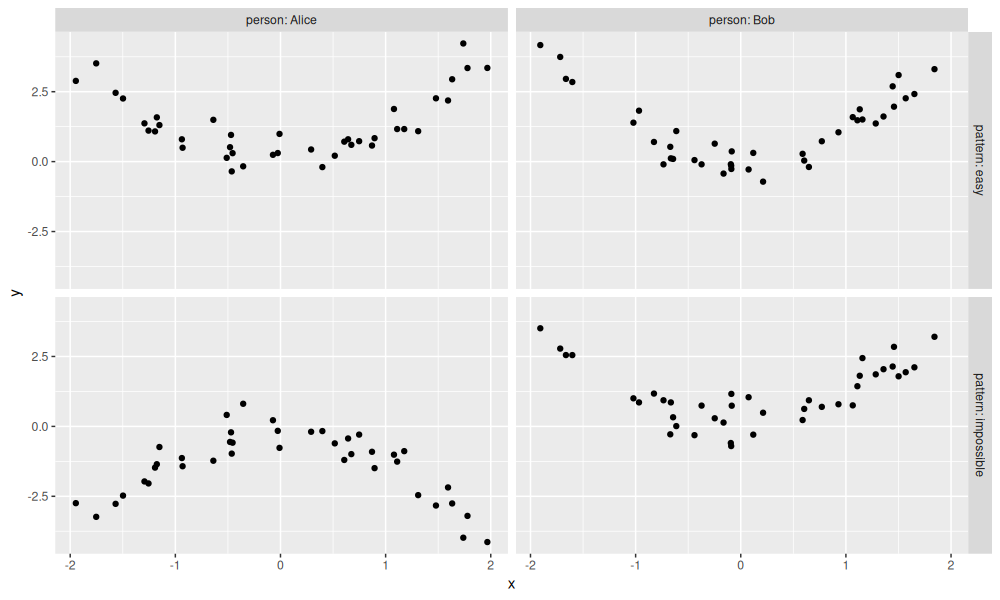
The figure above shows data for two simulated patterns:
- easy (top) has same pattern in the two people.
- impossible (bottom) has different patterns in the two people.
mlr3 benchmark grid
To use mlr3 on these data, we create a benchmark grid with a list of tasks and learners in the code below.
reg.learner.list <- list(
  featureless=mlr3::LearnerRegrFeatureless$new())
if(requireNamespace("rpart")){
  reg.learner.list$rpart <- mlr3::LearnerRegrRpart$new()
}
(bench.grid <- mlr3::benchmark_grid(
  reg.task.list,
  reg.learner.list,
  SOAK))
##          task          learner          resampling
##        <char>           <char>              <char>
## 1:       easy regr.featureless same_other_sizes_cv
## 2:       easy       regr.rpart same_other_sizes_cv
## 3: impossible regr.featureless same_other_sizes_cv
## 4: impossible       regr.rpart same_other_sizes_cv
The output above indicates that we want to run same_other_sizes_cv
resampling on two different tasks, and two different learners.
To run that in sequence, we use the typical mlr3 functions in the code below.
lgr::get_logger("mlr3")$set_threshold("warn")
bench.result <- mlr3::benchmark(bench.grid)
bench.score <- mlr3resampling::score(bench.result, mlr3::msr("regr.rmse"))
bench.score[, .(task_id, algorithm, train.subsets, test.fold, test.subset, regr.rmse)]
##        task_id   algorithm train.subsets test.fold test.subset regr.rmse
##         <char>      <char>        <char>     <int>      <fctr>     <num>
##  1:       easy featureless           all         1       Alice 0.8417981
##  2:       easy featureless           all         1         Bob 1.4748311
##  3:       easy featureless           all         2       Alice 1.3892457
##  4:       easy featureless           all         2         Bob 1.2916491
##  5:       easy featureless           all         3       Alice 1.1636785
##  6:       easy featureless           all         3         Bob 1.0491199
##  7:       easy featureless         other         1       Alice 0.8559209
##  8:       easy featureless         other         1         Bob 1.4567103
##  9:       easy featureless         other         2       Alice 1.3736439
## 10:       easy featureless         other         2         Bob 1.2943787
## 11:       easy featureless         other         3       Alice 1.1395756
## 12:       easy featureless         other         3         Bob 1.0899069
## 13:       easy featureless          same         1       Alice 0.8667528
## 14:       easy featureless          same         1         Bob 1.5148801
## 15:       easy featureless          same         2       Alice 1.4054366
## 16:       easy featureless          same         2         Bob 1.2897447
## 17:       easy featureless          same         3       Alice 1.1917033
## 18:       easy featureless          same         3         Bob 1.0118805
## 19:       easy       rpart           all         1       Alice 0.6483484
## 20:       easy       rpart           all         1         Bob 0.5780414
## 21:       easy       rpart           all         2       Alice 0.7737929
## 22:       easy       rpart           all         2         Bob 0.6693803
## 23:       easy       rpart           all         3       Alice 0.4360203
## 24:       easy       rpart           all         3         Bob 0.5599774
## 25:       easy       rpart         other         1       Alice 0.7000487
## 26:       easy       rpart         other         1         Bob 1.3295572
## 27:       easy       rpart         other         2       Alice 1.2688572
## 28:       easy       rpart         other         2         Bob 0.9847977
## 29:       easy       rpart         other         3       Alice 0.8686188
## 30:       easy       rpart         other         3         Bob 0.8957394
## 31:       easy       rpart          same         1       Alice 0.9762360
## 32:       easy       rpart          same         1         Bob 1.3404500
## 33:       easy       rpart          same         2       Alice 1.1213335
## 34:       easy       rpart          same         2         Bob 1.1853491
## 35:       easy       rpart          same         3       Alice 0.7931738
## 36:       easy       rpart          same         3         Bob 0.9980859
## 37: impossible featureless           all         1       Alice 1.8015752
## 38: impossible featureless           all         1         Bob 2.0459690
## 39: impossible featureless           all         2       Alice 1.9332069
## 40: impossible featureless           all         2         Bob 1.3513960
## 41: impossible featureless           all         3       Alice 1.4087384
## 42: impossible featureless           all         3         Bob 1.5117399
## 43: impossible featureless         other         1       Alice 2.7435334
## 44: impossible featureless         other         1         Bob 3.0650008
## 45: impossible featureless         other         2       Alice 3.0673372
## 46: impossible featureless         other         2         Bob 2.4200628
## 47: impossible featureless         other         3       Alice 2.5631614
## 48: impossible featureless         other         3         Bob 2.7134959
## 49: impossible featureless          same         1       Alice 1.1982239
## 50: impossible featureless          same         1         Bob 1.2037929
## 51: impossible featureless          same         2       Alice 1.2865945
## 52: impossible featureless          same         2         Bob 1.1769211
## 53: impossible featureless          same         3       Alice 1.0677617
## 54: impossible featureless          same         3         Bob 0.9738987
## 55: impossible       rpart           all         1       Alice 1.9942054
## 56: impossible       rpart           all         1         Bob 2.9047858
## 57: impossible       rpart           all         2       Alice 1.9339810
## 58: impossible       rpart           all         2         Bob 1.6467536
## 59: impossible       rpart           all         3       Alice 1.6622025
## 60: impossible       rpart           all         3         Bob 1.7632037
## 61: impossible       rpart         other         1       Alice 2.9498727
## 62: impossible       rpart         other         1         Bob 3.0738533
## 63: impossible       rpart         other         2       Alice 3.5994187
## 64: impossible       rpart         other         2         Bob 2.9526543
## 65: impossible       rpart         other         3       Alice 2.5892647
## 66: impossible       rpart         other         3         Bob 3.1410587
## 67: impossible       rpart          same         1       Alice 0.9056522
## 68: impossible       rpart          same         1         Bob 1.3881235
## 69: impossible       rpart          same         2       Alice 0.8927662
## 70: impossible       rpart          same         2         Bob 0.7149474
## 71: impossible       rpart          same         3       Alice 0.9229746
## 72: impossible       rpart          same         3         Bob 0.6295206
##        task_id   algorithm train.subsets test.fold test.subset regr.rmse
##         <char>      <char>        <char>     <int>      <fctr>     <num>
The table of scores above shows the root mean squared error for each combination of task, algorithm, train subset, test fold, and test subset. These error values are summarized in the visualization below.
bench.plist <- mlr3resampling::pvalue(bench.score)
plot(bench.plist)
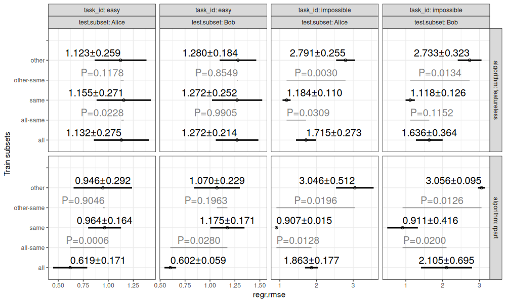
The figure above shows:
- in black, mean plus or minus standard deviation, for each combination of task, test subset, algorithm, and train subsets.
- in grey, P-values for differences between same/all and same/other (two-sided paired T-test).
Exercise for the reader: use the code above to do the computation in
parallel on your laptop, by first declaring future::plan("multisession").
Proposed method for expanding the ML grid
To run the same computations in parallel, we will create a data table with one row per train/test split, then compute these split results in parallel.
my.grid <- list(
  task_list=reg.task.list,
  learner_list=reg.learner.list,
  resampling=SOAK)
seq.proj.dir <- tempfile()
dir.create(seq.proj.dir)
saveRDS(my.grid, file.path(seq.proj.dir, "grid.rds"))
The code above saves a grid of tasks, learners, and a resampling to
the grid.rds file, in a project directory called seq.proj.dir
(because this first demonstration will be computation in sequence, not
parallel). Next, we create the table with one row per split to
compute,
proj_grid_jobs <- function(proj.dir){
  grid.rds <- file.path(proj.dir, "grid.rds")
  proj.grid <- readRDS(grid.rds)
  ml_job_dt_list <- list()
  for(task.name in names(proj.grid$task_list)){
    task.obj <- proj.grid$task_list[[task.name]]
    proj.grid$resampling$instantiate(task.obj)
    for(learner.name in names(proj.grid$learner_list)){
      ml_job_dt_list[[paste(task.name, learner.name)]] <- data.table(
        task.name, learner.name, iteration=seq_len(proj.grid$resampling$iters), status="not started")
    }
  }
  ml_job_dt <- rbindlist(ml_job_dt_list)
  grid_jobs.csv <- file.path(proj.dir, "grid_jobs.csv")
  fwrite(ml_job_dt, grid_jobs.csv)
  ml_job_dt
}
proj_grid_jobs(seq.proj.dir)
##      task.name learner.name iteration      status
##         <char>       <char>     <int>      <char>
##  1:       easy  featureless         1 not started
##  2:       easy  featureless         2 not started
##  3:       easy  featureless         3 not started
##  4:       easy  featureless         4 not started
##  5:       easy  featureless         5 not started
##  6:       easy  featureless         6 not started
##  7:       easy  featureless         7 not started
##  8:       easy  featureless         8 not started
##  9:       easy  featureless         9 not started
## 10:       easy  featureless        10 not started
## 11:       easy  featureless        11 not started
## 12:       easy  featureless        12 not started
## 13:       easy  featureless        13 not started
## 14:       easy  featureless        14 not started
## 15:       easy  featureless        15 not started
## 16:       easy  featureless        16 not started
## 17:       easy  featureless        17 not started
## 18:       easy  featureless        18 not started
## 19:       easy        rpart         1 not started
## 20:       easy        rpart         2 not started
## 21:       easy        rpart         3 not started
## 22:       easy        rpart         4 not started
## 23:       easy        rpart         5 not started
## 24:       easy        rpart         6 not started
## 25:       easy        rpart         7 not started
## 26:       easy        rpart         8 not started
## 27:       easy        rpart         9 not started
## 28:       easy        rpart        10 not started
## 29:       easy        rpart        11 not started
## 30:       easy        rpart        12 not started
## 31:       easy        rpart        13 not started
## 32:       easy        rpart        14 not started
## 33:       easy        rpart        15 not started
## 34:       easy        rpart        16 not started
## 35:       easy        rpart        17 not started
## 36:       easy        rpart        18 not started
## 37: impossible  featureless         1 not started
## 38: impossible  featureless         2 not started
## 39: impossible  featureless         3 not started
## 40: impossible  featureless         4 not started
## 41: impossible  featureless         5 not started
## 42: impossible  featureless         6 not started
## 43: impossible  featureless         7 not started
## 44: impossible  featureless         8 not started
## 45: impossible  featureless         9 not started
## 46: impossible  featureless        10 not started
## 47: impossible  featureless        11 not started
## 48: impossible  featureless        12 not started
## 49: impossible  featureless        13 not started
## 50: impossible  featureless        14 not started
## 51: impossible  featureless        15 not started
## 52: impossible  featureless        16 not started
## 53: impossible  featureless        17 not started
## 54: impossible  featureless        18 not started
## 55: impossible        rpart         1 not started
## 56: impossible        rpart         2 not started
## 57: impossible        rpart         3 not started
## 58: impossible        rpart         4 not started
## 59: impossible        rpart         5 not started
## 60: impossible        rpart         6 not started
## 61: impossible        rpart         7 not started
## 62: impossible        rpart         8 not started
## 63: impossible        rpart         9 not started
## 64: impossible        rpart        10 not started
## 65: impossible        rpart        11 not started
## 66: impossible        rpart        12 not started
## 67: impossible        rpart        13 not started
## 68: impossible        rpart        14 not started
## 69: impossible        rpart        15 not started
## 70: impossible        rpart        16 not started
## 71: impossible        rpart        17 not started
## 72: impossible        rpart        18 not started
##      task.name learner.name iteration      status
##         <char>       <char>     <int>      <char>
In the output above, there is one row per train/test split (ML job). It includes every combination of task, learner, and cross-validation iteration. After saving these data to disk above, we can compute one result using the function below.
proj_compute <- function(proj.dir){
  library(data.table)
  grid_jobs.csv <- file.path(proj.dir, "grid_jobs.csv")
  grid_jobs.csv.lock <- paste0(grid_jobs.csv, ".lock")
  before.lock <- filelock::lock(grid_jobs.csv.lock)
  grid_jobs_dt <- fread(grid_jobs.csv)
  not.started <- grid_jobs_dt$status == "not started"
  grid_job_i <- NULL
  if(any(not.started)){
    grid_job_i <- which(not.started)[1]
    grid_jobs_dt[grid_job_i, status := "started"]
    fwrite(grid_jobs_dt, grid_jobs.csv)
  }
  filelock::unlock(before.lock)
  if(!is.null(grid_job_i)){
    start.time <- Sys.time()
    grid_job_row <- grid_jobs_dt[grid_job_i]
    grid.rds <- file.path(proj.dir, "grid.rds")
    proj.grid <- readRDS(grid.rds)
    this.task <- proj.grid$task_list[[grid_job_row$task.name]]
    this.learner <- proj.grid$learner_list[[grid_job_row$learner.name]]
    proj.grid$resampling$instantiate(this.task)
    set_rows <- function(train_or_test){
      train_or_test_set <- paste0(train_or_test, "_set")
      set_fun <- proj.grid$resampling[[train_or_test_set]]
      set_fun(grid_job_row$iteration)
    }
    this.learner$train(this.task, set_rows("train"))
    pred <- this.learner$predict(this.task, set_rows("test"))
    result.row <- data.table(
      grid_job_row,
      start.time, end.time=Sys.time(), process=Sys.getpid(),
      learner=list(this.learner),
      pred=list(pred))
    result.rds <- file.path(proj.dir, "grid_jobs", paste0(grid_job_i, ".rds"))
    dir.create(dirname(result.rds), showWarnings = FALSE)
    saveRDS(result.row, result.rds)
    result.row
  }
}
proj_compute(seq.proj.dir)
##    task.name learner.name iteration  status          start.time            end.time process
##       <char>       <char>     <int>  <char>              <POSc>              <POSc>   <int>
## 1:      easy  featureless         1 started 2025-06-23 12:14:36 2025-06-23 12:14:36 1585847
##                                      learner             pred
##                                       <list>           <list>
## 1: <LearnerRegrFeatureless:regr.featureless> <PredictionRegr>
proj_compute(seq.proj.dir)
##    task.name learner.name iteration  status          start.time            end.time process
##       <char>       <char>     <int>  <char>              <POSc>              <POSc>   <int>
## 1:      easy  featureless         2 started 2025-06-23 12:14:36 2025-06-23 12:14:36 1585847
##                                      learner             pred
##                                       <list>           <list>
## 1: <LearnerRegrFeatureless:regr.featureless> <PredictionRegr>
The output above show the results for two iterations. Each call to
proj_compute does the following:
- looks in the project directory and gets a lock on the
grid_jobs.csvfile, - checks if there are any splits that have not yet started,
- if any have not yet started, we select the next index,
grid_job_i, to compute next. - we look in
grid.rdsfor the correspond task, learner, and split, - after calling
train()andpredict(), we save the results to a RDS file. - Importantly, each call to
proj_compute()only specifies the directory to look in, not the particular split to compute. So at first, each process does not know what work to do, nor if there is any work to do at all! It looks at the file system to determine what work to do, if any.
Next, we use a while loop in the function below to keep going until there is no more work to do.
proj_compute_until_done <- function(proj.dir){
  done <- FALSE
  while(!done){
    result <- proj_compute(proj.dir)
    if(is.null(result))done <- TRUE
  }
}
proj_compute_until_done(seq.proj.dir)
Next, we look at the file system and combine the result files.
proj_results <- function(proj.dir){
  rbindlist(lapply(Sys.glob(file.path(proj.dir, "grid_jobs", "*.rds")), readRDS))
}
proj_results(seq.proj.dir)
##      task.name learner.name iteration  status          start.time            end.time process
##         <char>       <char>     <int>  <char>              <POSc>              <POSc>   <int>
##  1:       easy  featureless        10 started 2025-06-23 12:14:36 2025-06-23 12:14:36 1585847
##  2:       easy  featureless        11 started 2025-06-23 12:14:36 2025-06-23 12:14:36 1585847
##  3:       easy  featureless        12 started 2025-06-23 12:14:36 2025-06-23 12:14:36 1585847
##  4:       easy  featureless        13 started 2025-06-23 12:14:36 2025-06-23 12:14:37 1585847
##  5:       easy  featureless        14 started 2025-06-23 12:14:37 2025-06-23 12:14:37 1585847
##  6:       easy  featureless        15 started 2025-06-23 12:14:37 2025-06-23 12:14:37 1585847
##  7:       easy  featureless        16 started 2025-06-23 12:14:37 2025-06-23 12:14:37 1585847
##  8:       easy  featureless        17 started 2025-06-23 12:14:37 2025-06-23 12:14:37 1585847
##  9:       easy  featureless        18 started 2025-06-23 12:14:37 2025-06-23 12:14:37 1585847
## 10:       easy        rpart         1 started 2025-06-23 12:14:37 2025-06-23 12:14:37 1585847
## 11:       easy  featureless         1 started 2025-06-23 12:14:36 2025-06-23 12:14:36 1585847
## 12:       easy        rpart         2 started 2025-06-23 12:14:37 2025-06-23 12:14:37 1585847
## 13:       easy        rpart         3 started 2025-06-23 12:14:37 2025-06-23 12:14:37 1585847
## 14:       easy        rpart         4 started 2025-06-23 12:14:37 2025-06-23 12:14:37 1585847
## 15:       easy        rpart         5 started 2025-06-23 12:14:37 2025-06-23 12:14:37 1585847
## 16:       easy        rpart         6 started 2025-06-23 12:14:37 2025-06-23 12:14:37 1585847
## 17:       easy        rpart         7 started 2025-06-23 12:14:37 2025-06-23 12:14:38 1585847
## 18:       easy        rpart         8 started 2025-06-23 12:14:38 2025-06-23 12:14:38 1585847
## 19:       easy        rpart         9 started 2025-06-23 12:14:38 2025-06-23 12:14:38 1585847
## 20:       easy        rpart        10 started 2025-06-23 12:14:38 2025-06-23 12:14:38 1585847
## 21:       easy        rpart        11 started 2025-06-23 12:14:38 2025-06-23 12:14:38 1585847
## 22:       easy  featureless         2 started 2025-06-23 12:14:36 2025-06-23 12:14:36 1585847
## 23:       easy        rpart        12 started 2025-06-23 12:14:38 2025-06-23 12:14:38 1585847
## 24:       easy        rpart        13 started 2025-06-23 12:14:38 2025-06-23 12:14:38 1585847
## 25:       easy        rpart        14 started 2025-06-23 12:14:38 2025-06-23 12:14:38 1585847
## 26:       easy        rpart        15 started 2025-06-23 12:14:38 2025-06-23 12:14:38 1585847
## 27:       easy        rpart        16 started 2025-06-23 12:14:38 2025-06-23 12:14:38 1585847
## 28:       easy        rpart        17 started 2025-06-23 12:14:38 2025-06-23 12:14:38 1585847
## 29:       easy        rpart        18 started 2025-06-23 12:14:38 2025-06-23 12:14:39 1585847
## 30: impossible  featureless         1 started 2025-06-23 12:14:39 2025-06-23 12:14:39 1585847
## 31: impossible  featureless         2 started 2025-06-23 12:14:39 2025-06-23 12:14:39 1585847
## 32: impossible  featureless         3 started 2025-06-23 12:14:39 2025-06-23 12:14:39 1585847
## 33:       easy  featureless         3 started 2025-06-23 12:14:36 2025-06-23 12:14:36 1585847
## 34: impossible  featureless         4 started 2025-06-23 12:14:39 2025-06-23 12:14:39 1585847
## 35: impossible  featureless         5 started 2025-06-23 12:14:39 2025-06-23 12:14:39 1585847
## 36: impossible  featureless         6 started 2025-06-23 12:14:39 2025-06-23 12:14:39 1585847
## 37: impossible  featureless         7 started 2025-06-23 12:14:39 2025-06-23 12:14:39 1585847
## 38: impossible  featureless         8 started 2025-06-23 12:14:39 2025-06-23 12:14:39 1585847
## 39: impossible  featureless         9 started 2025-06-23 12:14:39 2025-06-23 12:14:39 1585847
## 40: impossible  featureless        10 started 2025-06-23 12:14:39 2025-06-23 12:14:40 1585847
## 41: impossible  featureless        11 started 2025-06-23 12:14:40 2025-06-23 12:14:40 1585847
## 42: impossible  featureless        12 started 2025-06-23 12:14:40 2025-06-23 12:14:40 1585847
## 43: impossible  featureless        13 started 2025-06-23 12:14:40 2025-06-23 12:14:40 1585847
## 44:       easy  featureless         4 started 2025-06-23 12:14:36 2025-06-23 12:14:36 1585847
## 45: impossible  featureless        14 started 2025-06-23 12:14:40 2025-06-23 12:14:40 1585847
## 46: impossible  featureless        15 started 2025-06-23 12:14:40 2025-06-23 12:14:40 1585847
## 47: impossible  featureless        16 started 2025-06-23 12:14:40 2025-06-23 12:14:40 1585847
## 48: impossible  featureless        17 started 2025-06-23 12:14:40 2025-06-23 12:14:40 1585847
## 49: impossible  featureless        18 started 2025-06-23 12:14:40 2025-06-23 12:14:40 1585847
## 50: impossible        rpart         1 started 2025-06-23 12:14:40 2025-06-23 12:14:40 1585847
## 51: impossible        rpart         2 started 2025-06-23 12:14:40 2025-06-23 12:14:40 1585847
## 52: impossible        rpart         3 started 2025-06-23 12:14:40 2025-06-23 12:14:41 1585847
## 53: impossible        rpart         4 started 2025-06-23 12:14:41 2025-06-23 12:14:41 1585847
## 54: impossible        rpart         5 started 2025-06-23 12:14:41 2025-06-23 12:14:41 1585847
## 55:       easy  featureless         5 started 2025-06-23 12:14:36 2025-06-23 12:14:36 1585847
## 56: impossible        rpart         6 started 2025-06-23 12:14:41 2025-06-23 12:14:41 1585847
## 57: impossible        rpart         7 started 2025-06-23 12:14:41 2025-06-23 12:14:41 1585847
## 58: impossible        rpart         8 started 2025-06-23 12:14:41 2025-06-23 12:14:41 1585847
## 59: impossible        rpart         9 started 2025-06-23 12:14:41 2025-06-23 12:14:41 1585847
## 60: impossible        rpart        10 started 2025-06-23 12:14:41 2025-06-23 12:14:41 1585847
## 61: impossible        rpart        11 started 2025-06-23 12:14:41 2025-06-23 12:14:41 1585847
## 62: impossible        rpart        12 started 2025-06-23 12:14:41 2025-06-23 12:14:41 1585847
## 63: impossible        rpart        13 started 2025-06-23 12:14:41 2025-06-23 12:14:42 1585847
## 64: impossible        rpart        14 started 2025-06-23 12:14:42 2025-06-23 12:14:42 1585847
## 65: impossible        rpart        15 started 2025-06-23 12:14:42 2025-06-23 12:14:42 1585847
## 66:       easy  featureless         6 started 2025-06-23 12:14:36 2025-06-23 12:14:36 1585847
## 67: impossible        rpart        16 started 2025-06-23 12:14:42 2025-06-23 12:14:42 1585847
## 68: impossible        rpart        17 started 2025-06-23 12:14:42 2025-06-23 12:14:42 1585847
## 69: impossible        rpart        18 started 2025-06-23 12:14:42 2025-06-23 12:14:42 1585847
## 70:       easy  featureless         7 started 2025-06-23 12:14:36 2025-06-23 12:14:36 1585847
## 71:       easy  featureless         8 started 2025-06-23 12:14:36 2025-06-23 12:14:36 1585847
## 72:       easy  featureless         9 started 2025-06-23 12:14:36 2025-06-23 12:14:36 1585847
##      task.name learner.name iteration  status          start.time            end.time process
##         <char>       <char>     <int>  <char>              <POSc>              <POSc>   <int>
##                                       learner             pred
##                                        <list>           <list>
##  1: <LearnerRegrFeatureless:regr.featureless> <PredictionRegr>
##  2: <LearnerRegrFeatureless:regr.featureless> <PredictionRegr>
##  3: <LearnerRegrFeatureless:regr.featureless> <PredictionRegr>
##  4: <LearnerRegrFeatureless:regr.featureless> <PredictionRegr>
##  5: <LearnerRegrFeatureless:regr.featureless> <PredictionRegr>
##  6: <LearnerRegrFeatureless:regr.featureless> <PredictionRegr>
##  7: <LearnerRegrFeatureless:regr.featureless> <PredictionRegr>
##  8: <LearnerRegrFeatureless:regr.featureless> <PredictionRegr>
##  9: <LearnerRegrFeatureless:regr.featureless> <PredictionRegr>
## 10:             <LearnerRegrRpart:regr.rpart> <PredictionRegr>
## 11: <LearnerRegrFeatureless:regr.featureless> <PredictionRegr>
## 12:             <LearnerRegrRpart:regr.rpart> <PredictionRegr>
## 13:             <LearnerRegrRpart:regr.rpart> <PredictionRegr>
## 14:             <LearnerRegrRpart:regr.rpart> <PredictionRegr>
## 15:             <LearnerRegrRpart:regr.rpart> <PredictionRegr>
## 16:             <LearnerRegrRpart:regr.rpart> <PredictionRegr>
## 17:             <LearnerRegrRpart:regr.rpart> <PredictionRegr>
## 18:             <LearnerRegrRpart:regr.rpart> <PredictionRegr>
## 19:             <LearnerRegrRpart:regr.rpart> <PredictionRegr>
## 20:             <LearnerRegrRpart:regr.rpart> <PredictionRegr>
## 21:             <LearnerRegrRpart:regr.rpart> <PredictionRegr>
## 22: <LearnerRegrFeatureless:regr.featureless> <PredictionRegr>
## 23:             <LearnerRegrRpart:regr.rpart> <PredictionRegr>
## 24:             <LearnerRegrRpart:regr.rpart> <PredictionRegr>
## 25:             <LearnerRegrRpart:regr.rpart> <PredictionRegr>
## 26:             <LearnerRegrRpart:regr.rpart> <PredictionRegr>
## 27:             <LearnerRegrRpart:regr.rpart> <PredictionRegr>
## 28:             <LearnerRegrRpart:regr.rpart> <PredictionRegr>
## 29:             <LearnerRegrRpart:regr.rpart> <PredictionRegr>
## 30: <LearnerRegrFeatureless:regr.featureless> <PredictionRegr>
## 31: <LearnerRegrFeatureless:regr.featureless> <PredictionRegr>
## 32: <LearnerRegrFeatureless:regr.featureless> <PredictionRegr>
## 33: <LearnerRegrFeatureless:regr.featureless> <PredictionRegr>
## 34: <LearnerRegrFeatureless:regr.featureless> <PredictionRegr>
## 35: <LearnerRegrFeatureless:regr.featureless> <PredictionRegr>
## 36: <LearnerRegrFeatureless:regr.featureless> <PredictionRegr>
## 37: <LearnerRegrFeatureless:regr.featureless> <PredictionRegr>
## 38: <LearnerRegrFeatureless:regr.featureless> <PredictionRegr>
## 39: <LearnerRegrFeatureless:regr.featureless> <PredictionRegr>
## 40: <LearnerRegrFeatureless:regr.featureless> <PredictionRegr>
## 41: <LearnerRegrFeatureless:regr.featureless> <PredictionRegr>
## 42: <LearnerRegrFeatureless:regr.featureless> <PredictionRegr>
## 43: <LearnerRegrFeatureless:regr.featureless> <PredictionRegr>
## 44: <LearnerRegrFeatureless:regr.featureless> <PredictionRegr>
## 45: <LearnerRegrFeatureless:regr.featureless> <PredictionRegr>
## 46: <LearnerRegrFeatureless:regr.featureless> <PredictionRegr>
## 47: <LearnerRegrFeatureless:regr.featureless> <PredictionRegr>
## 48: <LearnerRegrFeatureless:regr.featureless> <PredictionRegr>
## 49: <LearnerRegrFeatureless:regr.featureless> <PredictionRegr>
## 50:             <LearnerRegrRpart:regr.rpart> <PredictionRegr>
## 51:             <LearnerRegrRpart:regr.rpart> <PredictionRegr>
## 52:             <LearnerRegrRpart:regr.rpart> <PredictionRegr>
## 53:             <LearnerRegrRpart:regr.rpart> <PredictionRegr>
## 54:             <LearnerRegrRpart:regr.rpart> <PredictionRegr>
## 55: <LearnerRegrFeatureless:regr.featureless> <PredictionRegr>
## 56:             <LearnerRegrRpart:regr.rpart> <PredictionRegr>
## 57:             <LearnerRegrRpart:regr.rpart> <PredictionRegr>
## 58:             <LearnerRegrRpart:regr.rpart> <PredictionRegr>
## 59:             <LearnerRegrRpart:regr.rpart> <PredictionRegr>
## 60:             <LearnerRegrRpart:regr.rpart> <PredictionRegr>
## 61:             <LearnerRegrRpart:regr.rpart> <PredictionRegr>
## 62:             <LearnerRegrRpart:regr.rpart> <PredictionRegr>
## 63:             <LearnerRegrRpart:regr.rpart> <PredictionRegr>
## 64:             <LearnerRegrRpart:regr.rpart> <PredictionRegr>
## 65:             <LearnerRegrRpart:regr.rpart> <PredictionRegr>
## 66: <LearnerRegrFeatureless:regr.featureless> <PredictionRegr>
## 67:             <LearnerRegrRpart:regr.rpart> <PredictionRegr>
## 68:             <LearnerRegrRpart:regr.rpart> <PredictionRegr>
## 69:             <LearnerRegrRpart:regr.rpart> <PredictionRegr>
## 70: <LearnerRegrFeatureless:regr.featureless> <PredictionRegr>
## 71: <LearnerRegrFeatureless:regr.featureless> <PredictionRegr>
## 72: <LearnerRegrFeatureless:regr.featureless> <PredictionRegr>
##                                       learner             pred
##                                        <list>           <list>
Finally, we visualize the results.
norm_times <- function(DT)DT[, let(
  start.seconds=start.time-min(start.time),
  end.seconds=end.time-min(start.time),
  Process=factor(process)
)][]
result.list <- list()
process_viz <- function(name){
  DT <- result.list[[name]]
  ggplot()+
    ggtitle(name)+
    geom_segment(aes(
      start.seconds, Process,
      xend=end.seconds, yend=Process),
      data=DT)+
    geom_point(aes(
      end.seconds, Process),
      shape=1,
      data=DT)+
    scale_x_continuous("Seconds from start of computation")
}
result.list$laptop_sequential <- norm_times(proj_results(seq.proj.dir))
process_viz("laptop_sequential")
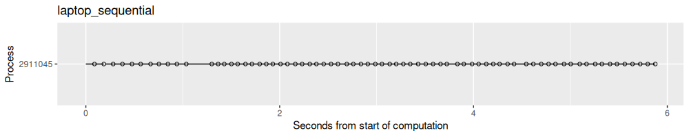
The output above shows each split as a dot (for end time) and line segment (which goes until the start time). It is clear that there was one process used to compute all of the results.
Laptop in parallel using batchtools
To compute in parallel, we can use batchtools.
We first setup a new project with a registry:
multi.proj.dir <- tempfile()
dir.create(multi.proj.dir)
saveRDS(my.grid, file.path(multi.proj.dir, "grid.rds"))
multi.job.dt <- proj_grid_jobs(multi.proj.dir)
reg.dir <- file.path(multi.proj.dir, "registry")
reg <- batchtools::makeRegistry(reg.dir)
## Sourcing configuration file '~/.batchtools.conf.R' ...
## Created registry in '/tmp/Rtmp3bxDpD/file1832b7584d8922/registry' using cluster functions 'Slurm'
reg$cluster.functions <- batchtools::makeClusterFunctionsMulticore()
## Auto-detected 14 CPUs
Note in the output above that we are using Multicore cluster functions. The code below launches the parallel computation in 2 worker processes.
n.workers <- 2
bm.jobs <- batchtools::batchMap(
  function(i)proj_compute_until_done(multi.proj.dir),
  seq(1, n.workers))
## Adding 2 jobs ...
batchtools::submitJobs(bm.jobs)
## Submitting 2 jobs in 2 chunks using cluster functions 'Multicore' ...
batchtools::waitForJobs()
##
## Waiting (Q::queued R::running D::done E::error ?::expired) [===========================================] 100% eta: 0s
## [1] TRUE
The code below visualizes the result.
result.list$laptop_multicore <- norm_times(proj_results(multi.proj.dir))
process_viz("laptop_multicore")
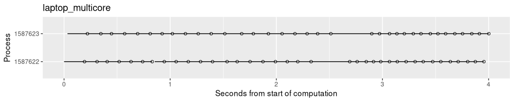
The output above shows that there are two processes working in parallel on the computation. After each process finishes a given split, it looks for a new split to work on, and starts right away (it does not have to wait for the other process to finish any work).
Using package functions
Based on the ideas in the functions above, I wrote some analogous functions in my mlr3resampling R package.
These functions allow runnning these kind of parallel ML experiments either locally, or on a SLURM compute cluster.
Below, we show how the local multi-core computation works.
pkg.proj.dir <- '2025-05-30-mlr3-filelock'
unlink(pkg.proj.dir, recursive=TRUE)
mlr3resampling::proj_grid(
  pkg.proj.dir,
  reg.task.list,
  reg.learner.list,
  SOAK,
  order_jobs = function(DT)DT[,order(test.subset)],
  score_args=mlr3::msrs(c("regr.rmse", "regr.mae")))
## task.i learner.i resampling.i task_id learner_id resampling_id test.subset train.subsets groups
## <int> <int> <int> <char> <char> <char> <fctr> <char> <int>
## 1: 1 1 1 easy regr.featureless same_other_sizes_cv Alice all 52
## 2: 1 1 1 easy regr.featureless same_other_sizes_cv Alice all 52
## 3: 1 1 1 easy regr.featureless same_other_sizes_cv Alice all 52
## 4: 1 1 1 easy regr.featureless same_other_sizes_cv Alice other 26
## 5: 1 1 1 easy regr.featureless same_other_sizes_cv Alice other 26
## 6: 1 1 1 easy regr.featureless same_other_sizes_cv Alice other 26
## 7: 1 1 1 easy regr.featureless same_other_sizes_cv Alice same 26
## 8: 1 1 1 easy regr.featureless same_other_sizes_cv Alice same 26
## 9: 1 1 1 easy regr.featureless same_other_sizes_cv Alice same 26
## 10: 1 2 1 easy regr.rpart same_other_sizes_cv Alice all 52
## 11: 1 2 1 easy regr.rpart same_other_sizes_cv Alice all 52
## 12: 1 2 1 easy regr.rpart same_other_sizes_cv Alice all 52
## 13: 1 2 1 easy regr.rpart same_other_sizes_cv Alice other 26
## 14: 1 2 1 easy regr.rpart same_other_sizes_cv Alice other 26
## 15: 1 2 1 easy regr.rpart same_other_sizes_cv Alice other 26
## 16: 1 2 1 easy regr.rpart same_other_sizes_cv Alice same 26
## 17: 1 2 1 easy regr.rpart same_other_sizes_cv Alice same 26
## 18: 1 2 1 easy regr.rpart same_other_sizes_cv Alice same 26
## 19: 2 1 1 impossible regr.featureless same_other_sizes_cv Alice all 52
## 20: 2 1 1 impossible regr.featureless same_other_sizes_cv Alice all 52
## 21: 2 1 1 impossible regr.featureless same_other_sizes_cv Alice all 52
## 22: 2 1 1 impossible regr.featureless same_other_sizes_cv Alice other 26
## 23: 2 1 1 impossible regr.featureless same_other_sizes_cv Alice other 26
## 24: 2 1 1 impossible regr.featureless same_other_sizes_cv Alice other 26
## 25: 2 1 1 impossible regr.featureless same_other_sizes_cv Alice same 26
## 26: 2 1 1 impossible regr.featureless same_other_sizes_cv Alice same 26
## 27: 2 1 1 impossible regr.featureless same_other_sizes_cv Alice same 26
## 28: 2 2 1 impossible regr.rpart same_other_sizes_cv Alice all 52
## 29: 2 2 1 impossible regr.rpart same_other_sizes_cv Alice all 52
## 30: 2 2 1 impossible regr.rpart same_other_sizes_cv Alice all 52
## 31: 2 2 1 impossible regr.rpart same_other_sizes_cv Alice other 26
## 32: 2 2 1 impossible regr.rpart same_other_sizes_cv Alice other 26
## 33: 2 2 1 impossible regr.rpart same_other_sizes_cv Alice other 26
## 34: 2 2 1 impossible regr.rpart same_other_sizes_cv Alice same 26
## 35: 2 2 1 impossible regr.rpart same_other_sizes_cv Alice same 26
## 36: 2 2 1 impossible regr.rpart same_other_sizes_cv Alice same 26
## 37: 1 1 1 easy regr.featureless same_other_sizes_cv Bob all 52
## 38: 1 1 1 easy regr.featureless same_other_sizes_cv Bob all 52
## 39: 1 1 1 easy regr.featureless same_other_sizes_cv Bob all 52
## 40: 1 1 1 easy regr.featureless same_other_sizes_cv Bob other 26
## 41: 1 1 1 easy regr.featureless same_other_sizes_cv Bob other 26
## 42: 1 1 1 easy regr.featureless same_other_sizes_cv Bob other 26
## 43: 1 1 1 easy regr.featureless same_other_sizes_cv Bob same 26
## 44: 1 1 1 easy regr.featureless same_other_sizes_cv Bob same 26
## 45: 1 1 1 easy regr.featureless same_other_sizes_cv Bob same 26
## 46: 1 2 1 easy regr.rpart same_other_sizes_cv Bob all 52
## 47: 1 2 1 easy regr.rpart same_other_sizes_cv Bob all 52
## 48: 1 2 1 easy regr.rpart same_other_sizes_cv Bob all 52
## 49: 1 2 1 easy regr.rpart same_other_sizes_cv Bob other 26
## 50: 1 2 1 easy regr.rpart same_other_sizes_cv Bob other 26
## 51: 1 2 1 easy regr.rpart same_other_sizes_cv Bob other 26
## 52: 1 2 1 easy regr.rpart same_other_sizes_cv Bob same 26
## 53: 1 2 1 easy regr.rpart same_other_sizes_cv Bob same 26
## 54: 1 2 1 easy regr.rpart same_other_sizes_cv Bob same 26
## 55: 2 1 1 impossible regr.featureless same_other_sizes_cv Bob all 52
## 56: 2 1 1 impossible regr.featureless same_other_sizes_cv Bob all 52
## 57: 2 1 1 impossible regr.featureless same_other_sizes_cv Bob all 52
## 58: 2 1 1 impossible regr.featureless same_other_sizes_cv Bob other 26
## 59: 2 1 1 impossible regr.featureless same_other_sizes_cv Bob other 26
## 60: 2 1 1 impossible regr.featureless same_other_sizes_cv Bob other 26
## 61: 2 1 1 impossible regr.featureless same_other_sizes_cv Bob same 26
## 62: 2 1 1 impossible regr.featureless same_other_sizes_cv Bob same 26
## 63: 2 1 1 impossible regr.featureless same_other_sizes_cv Bob same 26
## 64: 2 2 1 impossible regr.rpart same_other_sizes_cv Bob all 52
## 65: 2 2 1 impossible regr.rpart same_other_sizes_cv Bob all 52
## 66: 2 2 1 impossible regr.rpart same_other_sizes_cv Bob all 52
## 67: 2 2 1 impossible regr.rpart same_other_sizes_cv Bob other 26
## 68: 2 2 1 impossible regr.rpart same_other_sizes_cv Bob other 26
## 69: 2 2 1 impossible regr.rpart same_other_sizes_cv Bob other 26
## 70: 2 2 1 impossible regr.rpart same_other_sizes_cv Bob same 26
## 71: 2 2 1 impossible regr.rpart same_other_sizes_cv Bob same 26
## 72: 2 2 1 impossible regr.rpart same_other_sizes_cv Bob same 26
## task.i learner.i resampling.i task_id learner_id resampling_id test.subset train.subsets groups
## <int> <int> <int> <char> <char> <char> <fctr> <char> <int>
## test.fold test train seed n.train.groups iteration
## <int> <list> <list> <int> <int> <int>
## 1: 1 3, 4, 5,12,13,20,... 1,2,6,7,8,9,... 1 52 1
## 2: 2 1, 2, 8,10,11,17,... 3,4,5,6,7,9,... 1 52 3
## 3: 3 6, 7, 9,14,15,16,... 1,2,3,4,5,8,... 1 52 5
## 4: 1 3, 4, 5,12,13,20,... 41,42,43,44,47,52,... 1 26 7
## 5: 2 1, 2, 8,10,11,17,... 42,44,45,46,47,48,... 1 26 9
## 6: 3 6, 7, 9,14,15,16,... 41,43,45,46,48,49,... 1 26 11
## 7: 1 3, 4, 5,12,13,20,... 1,2,6,7,8,9,... 1 26 13
## 8: 2 1, 2, 8,10,11,17,... 3,4,5,6,7,9,... 1 26 15
## 9: 3 6, 7, 9,14,15,16,... 1,2,3,4,5,8,... 1 26 17
## 10: 1 3, 4, 5,12,13,20,... 1,2,6,7,8,9,... 1 52 1
## 11: 2 1, 2, 8,10,11,17,... 3,4,5,6,7,9,... 1 52 3
## 12: 3 6, 7, 9,14,15,16,... 1,2,3,4,5,8,... 1 52 5
## 13: 1 3, 4, 5,12,13,20,... 41,42,43,44,47,52,... 1 26 7
## 14: 2 1, 2, 8,10,11,17,... 42,44,45,46,47,48,... 1 26 9
## 15: 3 6, 7, 9,14,15,16,... 41,43,45,46,48,49,... 1 26 11
## 16: 1 3, 4, 5,12,13,20,... 1,2,6,7,8,9,... 1 26 13
## 17: 2 1, 2, 8,10,11,17,... 3,4,5,6,7,9,... 1 26 15
## 18: 3 6, 7, 9,14,15,16,... 1,2,3,4,5,8,... 1 26 17
## 19: 1 6, 7, 9,12,14,17,... 1,2,3,4,5,8,... 1 52 1
## 20: 2 1, 3, 4,18,19,20,... 2,5,6,7,8,9,... 1 52 3
## 21: 3 2, 5, 8,10,11,13,... 1,3,4,6,7,9,... 1 52 5
## 22: 1 6, 7, 9,12,14,17,... 41,43,44,45,46,49,... 1 26 7
## 23: 2 1, 3, 4,18,19,20,... 41,42,46,47,48,49,... 1 26 9
## 24: 3 2, 5, 8,10,11,13,... 42,43,44,45,47,48,... 1 26 11
## 25: 1 6, 7, 9,12,14,17,... 1,2,3,4,5,8,... 1 26 13
## 26: 2 1, 3, 4,18,19,20,... 2,5,6,7,8,9,... 1 26 15
## 27: 3 2, 5, 8,10,11,13,... 1,3,4,6,7,9,... 1 26 17
## 28: 1 6, 7, 9,12,14,17,... 1,2,3,4,5,8,... 1 52 1
## 29: 2 1, 3, 4,18,19,20,... 2,5,6,7,8,9,... 1 52 3
## 30: 3 2, 5, 8,10,11,13,... 1,3,4,6,7,9,... 1 52 5
## 31: 1 6, 7, 9,12,14,17,... 41,43,44,45,46,49,... 1 26 7
## 32: 2 1, 3, 4,18,19,20,... 41,42,46,47,48,49,... 1 26 9
## 33: 3 2, 5, 8,10,11,13,... 42,43,44,45,47,48,... 1 26 11
## 34: 1 6, 7, 9,12,14,17,... 1,2,3,4,5,8,... 1 26 13
## 35: 2 1, 3, 4,18,19,20,... 2,5,6,7,8,9,... 1 26 15
## 36: 3 2, 5, 8,10,11,13,... 1,3,4,6,7,9,... 1 26 17
## 37: 1 45,46,48,49,50,51,... 1,2,6,7,8,9,... 1 52 2
## 38: 2 41,43,52,56,57,58,... 3,4,5,6,7,9,... 1 52 4
## 39: 3 42,44,47,53,54,55,... 1,2,3,4,5,8,... 1 52 6
## 40: 1 45,46,48,49,50,51,... 1,2,6,7,8,9,... 1 26 8
## 41: 2 41,43,52,56,57,58,... 3,4,5,6,7,9,... 1 26 10
## 42: 3 42,44,47,53,54,55,... 1,2,3,4,5,8,... 1 26 12
## 43: 1 45,46,48,49,50,51,... 41,42,43,44,47,52,... 1 26 14
## 44: 2 41,43,52,56,57,58,... 42,44,45,46,47,48,... 1 26 16
## 45: 3 42,44,47,53,54,55,... 41,43,45,46,48,49,... 1 26 18
## 46: 1 45,46,48,49,50,51,... 1,2,6,7,8,9,... 1 52 2
## 47: 2 41,43,52,56,57,58,... 3,4,5,6,7,9,... 1 52 4
## 48: 3 42,44,47,53,54,55,... 1,2,3,4,5,8,... 1 52 6
## 49: 1 45,46,48,49,50,51,... 1,2,6,7,8,9,... 1 26 8
## 50: 2 41,43,52,56,57,58,... 3,4,5,6,7,9,... 1 26 10
## 51: 3 42,44,47,53,54,55,... 1,2,3,4,5,8,... 1 26 12
## 52: 1 45,46,48,49,50,51,... 41,42,43,44,47,52,... 1 26 14
## 53: 2 41,43,52,56,57,58,... 42,44,45,46,47,48,... 1 26 16
## 54: 3 42,44,47,53,54,55,... 41,43,45,46,48,49,... 1 26 18
## 55: 1 42,47,48,52,53,59,... 1,2,3,4,5,8,... 1 52 2
## 56: 2 43,44,45,50,55,56,... 2,5,6,7,8,9,... 1 52 4
## 57: 3 41,46,49,51,54,57,... 1,3,4,6,7,9,... 1 52 6
## 58: 1 42,47,48,52,53,59,... 1,2,3,4,5,8,... 1 26 8
## 59: 2 43,44,45,50,55,56,... 2,5,6,7,8,9,... 1 26 10
## 60: 3 41,46,49,51,54,57,... 1,3,4,6,7,9,... 1 26 12
## 61: 1 42,47,48,52,53,59,... 41,43,44,45,46,49,... 1 26 14
## 62: 2 43,44,45,50,55,56,... 41,42,46,47,48,49,... 1 26 16
## 63: 3 41,46,49,51,54,57,... 42,43,44,45,47,48,... 1 26 18
## 64: 1 42,47,48,52,53,59,... 1,2,3,4,5,8,... 1 52 2
## 65: 2 43,44,45,50,55,56,... 2,5,6,7,8,9,... 1 52 4
## 66: 3 41,46,49,51,54,57,... 1,3,4,6,7,9,... 1 52 6
## 67: 1 42,47,48,52,53,59,... 1,2,3,4,5,8,... 1 26 8
## 68: 2 43,44,45,50,55,56,... 2,5,6,7,8,9,... 1 26 10
## 69: 3 41,46,49,51,54,57,... 1,3,4,6,7,9,... 1 26 12
## 70: 1 42,47,48,52,53,59,... 41,43,44,45,46,49,... 1 26 14
## 71: 2 43,44,45,50,55,56,... 41,42,46,47,48,49,... 1 26 16
## 72: 3 41,46,49,51,54,57,... 42,43,44,45,47,48,... 1 26 18
## test.fold test train seed n.train.groups iteration
## <int> <list> <list> <int> <int> <int>
Above we create a new project based on the same grid as in previous sections.
Other arguments include order_jobs, which returns an integer vector that specifies the priority/order of execution of the different ML experiments. This could be useful for the situation where you run out of time on SLURM, in which case only the entries at the top of the table will have results on the file system. In that case, you can also use the order_jobs argument to resume work from where you left off (only provide the indices of arguments that have not yet completed).
mlr3resampling::proj_submit(pkg.proj.dir)
## Sourcing configuration file '~/.batchtools.conf.R' ...
## Created registry in '/home/local/USHERBROOKE/hoct2726/tdhock.github.io/_posts/2025-05-30-mlr3-filelock/registry' using cluster functions 'Slurm'
## Adding 2 jobs ...
## Submitting 2 jobs in 1 chunks using cluster functions 'Slurm' ...
## Job Registry
##   Backend  : Slurm
##   File dir : /home/local/USHERBROOKE/hoct2726/tdhock.github.io/_posts/2025-05-30-mlr3-filelock/registry
##   Work dir : /home/local/USHERBROOKE/hoct2726/tdhock.github.io/_posts
##   Jobs     : 2
##   Seed     : 31826
##   Writeable: TRUE
batchtools::waitForJobs()
##
## Waiting (Q::queued R::running D::done E::error ?::expired) [===========================================] 100% eta: 0s
## [1] TRUE
result.list$laptop_pkg <- norm_times(fread(file.path(pkg.proj.dir,"results.csv")))
process_viz("laptop_pkg")
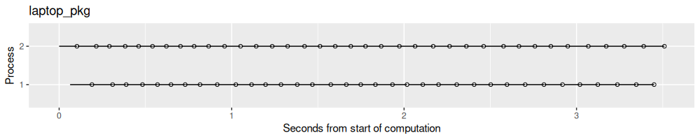
Above we see the result on my laptop. Below we see the results when using two SLURM clusters.
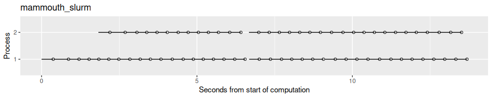
result.list$mammouth_slurm <- norm_times(fread("2025-05-30-mlr3-filelock-mammouth/results.csv"))
process_viz("mammouth_slurm")
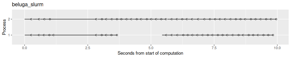
result.list$beluga_slurm <- norm_times(fread("2025-05-30-mlr3-filelock-beluga/results.csv"))
process_viz("beluga_slurm")
Compare them all
Here we compare the results for the different tests on the same plot.
common.names <- Reduce(intersect, sapply(result.list, names))
compare_results_list <- list()
for(computer in names(result.list)){
  compare_results_list[[computer]] <- data.table(
    computer,
    result.list[[computer]][, common.names, with=FALSE])
}
(compare_results <- rbindlist(compare_results_list))
##               computer iteration          start.time            end.time process  start.seconds    end.seconds Process
##                 <char>     <int>              <POSc>              <POSc>   <int>     <difftime>     <difftime>  <fctr>
##   1: laptop_sequential        10 2025-06-23 12:14:36 2025-06-23 12:14:36 1585847 0.7532570 secs 0.8191888 secs 1585847
##   2: laptop_sequential        11 2025-06-23 12:14:36 2025-06-23 12:14:36 1585847 0.8225505 secs 0.9087043 secs 1585847
##   3: laptop_sequential        12 2025-06-23 12:14:36 2025-06-23 12:14:36 1585847 0.9120812 secs 0.9776857 secs 1585847
##   4: laptop_sequential        13 2025-06-23 12:14:36 2025-06-23 12:14:37 1585847 0.9809139 secs 1.0681767 secs 1585847
##   5: laptop_sequential        14 2025-06-23 12:14:37 2025-06-23 12:14:37 1585847 1.0715811 secs 1.1556838 secs 1585847
##  ---
## 356:      beluga_slurm        10 2025-05-31 12:51:12 2025-05-31 12:51:12       2 9.3785510 secs 9.5612240 secs       2
## 357:      beluga_slurm        12 2025-05-31 12:51:12 2025-05-31 12:51:12       1 9.4658461 secs 9.6455581 secs       1
## 358:      beluga_slurm        14 2025-05-31 12:51:12 2025-05-31 12:51:12       2 9.5708041 secs 9.7502091 secs       2
## 359:      beluga_slurm        16 2025-05-31 12:51:12 2025-05-31 12:51:12       1 9.6548691 secs 9.8320482 secs       1
## 360:      beluga_slurm        18 2025-05-31 12:51:12 2025-05-31 12:51:13       2 9.7764421 secs 9.9576142 secs       2
ggplot()+
  geom_segment(aes(
    start.seconds, Process,
    xend=end.seconds, yend=Process),
    data=compare_results)+
  geom_point(aes(
    end.seconds, Process),
    shape=1,
    data=compare_results)+
  scale_x_continuous("Seconds from start of computation")+
  facet_grid(computer ~ ., scales="free")
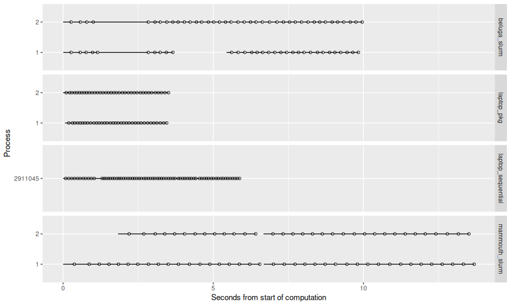
The figure above shows that the different computers have different timings. In particular, Mammouth seems to be quite a bit slower than the other methods (but it may be easier to get time on it).
A larger experiment
In typical machine learning experiments, the train and predict times
are much larger, because there are larger data sets, and more complex
learning algorithms. Below we analyze an experiment similar to the one
described in Comparing neural network architectures using
mlr3torch. It is
an analysis of a convolutional neural
network,
for the EMNIST_rot image pair data set, described in the SOAK
paper.
Below we read the result file.
old_dt <- fread("../assets/2025-05-30-mlr3-filelock-beluga/large-old.csv")
first <- min(old_dt$submitted)
hours <- function(x)difftime(x, first, units="hours")
old_dt[, let(
  Process=.I,
  submit.hours=hours(submitted),
  start.hours=hours(started),
  end.hours=hours(done)
)][]
##      job.id           submitted             started                done  error mem.used     batch.id
##       <int>              <POSc>              <POSc>              <POSc> <lgcl>   <lgcl>       <char>
##   1:      1 2025-03-25 12:04:45 2025-03-25 12:43:21 2025-03-25 21:20:00     NA       NA   54778789_1
##   2:      2 2025-03-25 12:04:45 2025-03-25 12:43:21 2025-03-25 21:30:57     NA       NA   54778789_2
##   3:      3 2025-03-25 12:04:45 2025-03-25 12:43:21 2025-03-25 21:13:02     NA       NA   54778789_3
##   4:      4 2025-03-25 12:04:45 2025-03-25 12:43:21 2025-03-25 21:01:17     NA       NA   54778789_4
##   5:      5 2025-03-25 12:04:45 2025-03-25 12:43:21 2025-03-25 21:30:58     NA       NA   54778789_5
##  ---
## 296:    296 2025-03-25 12:04:45 2025-03-25 14:24:46 2025-03-26 01:51:37     NA       NA 54778789_296
## 297:    297 2025-03-25 12:04:45 2025-03-25 14:24:24 2025-03-25 17:45:49     NA       NA 54778789_297
## 298:    298 2025-03-25 12:04:45 2025-03-25 14:24:04 2025-03-25 22:50:49     NA       NA 54778789_298
## 299:    299 2025-03-25 12:04:45 2025-03-25 14:24:24 2025-03-25 20:19:39     NA       NA 54778789_299
## 300:    300 2025-03-25 12:04:45 2025-03-25 14:24:24 2025-03-25 23:25:47     NA       NA 54778789_300
##                                         log.file                            job.hash
##                                           <char>                              <char>
##   1:   job77ad22aa390c5e2ebde0905bd77bffd1.log_1 job77ad22aa390c5e2ebde0905bd77bffd1
##   2:   job77ad22aa390c5e2ebde0905bd77bffd1.log_2 job77ad22aa390c5e2ebde0905bd77bffd1
##   3:   job77ad22aa390c5e2ebde0905bd77bffd1.log_3 job77ad22aa390c5e2ebde0905bd77bffd1
##   4:   job77ad22aa390c5e2ebde0905bd77bffd1.log_4 job77ad22aa390c5e2ebde0905bd77bffd1
##   5:   job77ad22aa390c5e2ebde0905bd77bffd1.log_5 job77ad22aa390c5e2ebde0905bd77bffd1
##  ---
## 296: job77ad22aa390c5e2ebde0905bd77bffd1.log_296 job77ad22aa390c5e2ebde0905bd77bffd1
## 297: job77ad22aa390c5e2ebde0905bd77bffd1.log_297 job77ad22aa390c5e2ebde0905bd77bffd1
## 298: job77ad22aa390c5e2ebde0905bd77bffd1.log_298 job77ad22aa390c5e2ebde0905bd77bffd1
## 299: job77ad22aa390c5e2ebde0905bd77bffd1.log_299 job77ad22aa390c5e2ebde0905bd77bffd1
## 300: job77ad22aa390c5e2ebde0905bd77bffd1.log_300 job77ad22aa390c5e2ebde0905bd77bffd1
##                                  job.name  repl time.queued time.running          problem   algorithm   tags
##                                    <char> <int>       <num>        <num>           <char>      <char> <lgcl>
##   1: 0f4f5711-194b-4ba2-bd7e-59de9097a907     1    2315.938     30999.48 ce2f347d4dd7afc8 run_learner     NA
##   2: 0f4f5711-194b-4ba2-bd7e-59de9097a907     2    2315.931     31656.00 ce2f347d4dd7afc8 run_learner     NA
##   3: 0f4f5711-194b-4ba2-bd7e-59de9097a907     3    2315.931     30580.57 ce2f347d4dd7afc8 run_learner     NA
##   4: 0f4f5711-194b-4ba2-bd7e-59de9097a907     4    2315.930     29876.11 ce2f347d4dd7afc8 run_learner     NA
##   5: 0f4f5711-194b-4ba2-bd7e-59de9097a907     5    2315.930     31657.44 ce2f347d4dd7afc8 run_learner     NA
##  ---
## 296: 968f2e00-601c-4ed8-9377-e5b65bb502ca    56    8400.745     41211.20 ce2f347d4dd7afc8 run_learner     NA
## 297: 968f2e00-601c-4ed8-9377-e5b65bb502ca    57    8379.287     12084.78 ce2f347d4dd7afc8 run_learner     NA
## 298: 968f2e00-601c-4ed8-9377-e5b65bb502ca    58    8359.098     30404.99 ce2f347d4dd7afc8 run_learner     NA
## 299: 968f2e00-601c-4ed8-9377-e5b65bb502ca    59    8379.310     21315.10 ce2f347d4dd7afc8 run_learner     NA
## 300: 968f2e00-601c-4ed8-9377-e5b65bb502ca    60    8379.294     32482.85 ce2f347d4dd7afc8 run_learner     NA
##               algo             task     start.hours       end.hours Process submit.hours
##             <char>           <char>      <difftime>      <difftime>   <int>   <difftime>
##   1:    torch_conv MNIST_EMNIST_rot 0.6433160 hours  9.254283 hours       1      0 hours
##   2:    torch_conv MNIST_EMNIST_rot 0.6433142 hours  9.436647 hours       2      0 hours
##   3:    torch_conv MNIST_EMNIST_rot 0.6433142 hours  9.137916 hours       3      0 hours
##   4:    torch_conv MNIST_EMNIST_rot 0.6433140 hours  8.942234 hours       4      0 hours
##   5:    torch_conv MNIST_EMNIST_rot 0.6433140 hours  9.437047 hours       5      0 hours
##  ---
## 296: cv_glmnet_min MNIST_EMNIST_rot 2.3335402 hours 13.781095 hours     296      0 hours
## 297: cv_glmnet_min MNIST_EMNIST_rot 2.3275798 hours  5.684464 hours     297      0 hours
## 298: cv_glmnet_min MNIST_EMNIST_rot 2.3219716 hours 10.767801 hours     298      0 hours
## 299: cv_glmnet_min MNIST_EMNIST_rot 2.3275862 hours  8.248448 hours     299      0 hours
## 300: cv_glmnet_min MNIST_EMNIST_rot 2.3275817 hours 11.350597 hours     300      0 hours
The data table above came from batchtools::getJobTable(), with a few
columns added for visualization of the parallel processing, which we do below.
old.not.na <- old_dt[!is.na(started)]
ggplot()+
  ggtitle(paste("mlr3batchmark::batchmark() nrow=", nrow(old.not.na)))+
  theme_bw()+
  geom_segment(aes(
    start.hours, Process,
    color=algo,
    xend=end.hours, yend=Process),
    data=old.not.na)+
  geom_point(aes(
    end.hours, Process,
    color=algo),
    shape=1,
    data=old.not.na)+
  scale_x_continuous(
    "Hours from submit time",
    breaks=seq(-100, 100, by=2),
    limits=c(0,16))
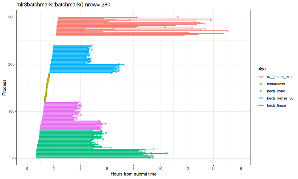
Above we see each train/test split as a line segment, with a dot at the end. We see there is only one line segment per Y/process value (300 total). Interestingly, we can see that the bottom third in each algo takes longer, because that corresponds to the All subset in SOAK (which has more rows than Same/Other).
Below we read in results of an attempt to use the
mlr3resampling::proj_*() functions to re-do this experiment.
large_dt <- fread("../assets/2025-05-30-mlr3-filelock-beluga/large.csv")
first <- min(large_dt$start.time)
hours <- function(x)difftime(x, first, units="hours")
large_dt[, let(
  start.hours=hours(start.time),
  end.hours=hours(end.time),
  Process=as.integer(factor(process))
)][]
##      task.i learner.i resampling.i iteration          start.time            end.time process          task.id
##       <int>     <int>        <int>     <int>              <POSc>              <POSc>   <int>           <char>
##   1:      1         1            1         1 2025-05-31 17:29:27 2025-05-31 17:29:35 2035134 MNIST_EMNIST_rot
##   2:      1         1            1         2 2025-05-31 17:31:36 2025-05-31 17:31:44 2035134 MNIST_EMNIST_rot
##   3:      1         1            1         3 2025-05-31 18:09:28 2025-05-31 18:09:44      58 MNIST_EMNIST_rot
##   4:      1         1            1         4 2025-05-31 18:09:28 2025-05-31 18:09:44      18 MNIST_EMNIST_rot
##   5:      1         1            1         5 2025-05-31 18:09:28 2025-05-31 18:09:44      85 MNIST_EMNIST_rot
##  ---
## 276:      1         5            1        56 2025-06-01 01:42:22 2025-06-01 12:48:44      99 MNIST_EMNIST_rot
## 277:      1         5            1        57 2025-06-01 01:44:54 2025-06-01 08:09:45      71 MNIST_EMNIST_rot
## 278:      1         5            1        58 2025-06-01 01:55:38 2025-06-01 12:33:55      29 MNIST_EMNIST_rot
## 279:      1         5            1        59 2025-06-01 01:58:26 2025-06-01 05:05:41      84 MNIST_EMNIST_rot
## 280:      1         5            1        60 2025-06-01 02:06:33 2025-06-01 13:01:36      92 MNIST_EMNIST_rot
##         learner.id       resampling.id test.subset train.subsets groups test.fold  seed n.train.groups     start.hours
##             <char>              <char>      <char>        <char>  <int>     <int> <int>          <int>      <difftime>
##   1:   featureless same_other_sizes_cv  EMNIST_rot           all 126000         1     1         126000 0.0000000 hours
##   2:   featureless same_other_sizes_cv       MNIST           all 126000         1     1         126000 0.0357750 hours
##   3:   featureless same_other_sizes_cv  EMNIST_rot           all 126000         2     1         126000 0.6668174 hours
##   4:   featureless same_other_sizes_cv       MNIST           all 126000         2     1         126000 0.6668216 hours
##   5:   featureless same_other_sizes_cv  EMNIST_rot           all 126000         3     1         126000 0.6668672 hours
##  ---
## 276: cv_glmnet_min same_other_sizes_cv       MNIST          same  63000         8     1          63000 8.2153686 hours
## 277: cv_glmnet_min same_other_sizes_cv  EMNIST_rot          same  63000         9     1          63000 8.2574947 hours
## 278: cv_glmnet_min same_other_sizes_cv       MNIST          same  63000         9     1          63000 8.4364010 hours
## 279: cv_glmnet_min same_other_sizes_cv  EMNIST_rot          same  63000        10     1          63000 8.4829044 hours
## 280: cv_glmnet_min same_other_sizes_cv       MNIST          same  63000        10     1          63000 8.6183932 hours
##               end.hours Process
##              <difftime>   <int>
##   1:  0.002151894 hours      96
##   2:  0.037924524 hours      96
##   3:  0.671318384 hours      55
##   4:  0.671368879 hours      16
##   5:  0.671334282 hours      81
##  ---
## 276: 19.321430867 hours      94
## 277: 14.671591418 hours      67
## 278: 19.074528557 hours      27
## 279: 11.603760343 hours      80
## 280: 19.535713733 hours      87
Above we see the result table, which is visualized along the time dimension below.
ggplot()+
  ggtitle(paste("mlr3resampling::proj_grid() nrow=", nrow(large_dt)))+
  theme_bw()+
  geom_segment(aes(
    start.hours, Process,
    color=learner.id,
    xend=end.hours, yend=Process),
    data=large_dt)+
  scale_fill_manual(values=c(
    same="white",
    other="grey",
    all="black"))+
  geom_point(aes(
    end.hours, Process,
    fill=train.subsets,
    color=learner.id),
    shape=21,
    data=large_dt)+
  scale_x_continuous(
    "Hours from submit time",
    breaks=seq(-100, 100, by=2))
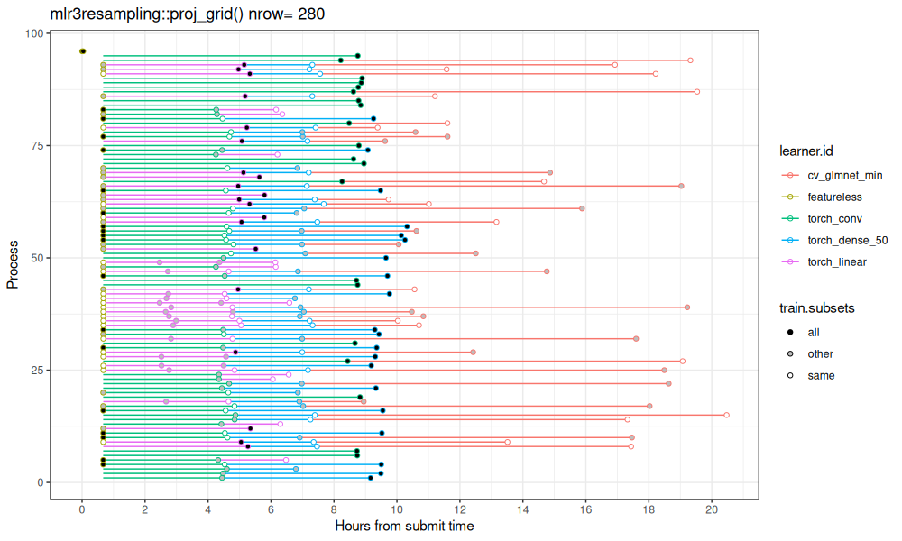
Above we see a different trend: there are multiple results computed in a single process.
Below we combine the results in the same plot.
(large_combined <- rbind(
  data.table(old.not.na[, .(
    pkg="mlr3batchmark", start.hours, end.hours, Process, learner.id=algo)]),
  data.table(large_dt[, .(
    pkg="mlr3resampling", start.hours, end.hours, Process, learner.id)])))
##                 pkg     start.hours       end.hours Process    learner.id
##              <char>      <difftime>      <difftime>   <int>        <char>
##   1:  mlr3batchmark 0.6433160 hours  9.254283 hours       1    torch_conv
##   2:  mlr3batchmark 0.6433142 hours  9.436647 hours       2    torch_conv
##   3:  mlr3batchmark 0.6433142 hours  9.137916 hours       3    torch_conv
##   4:  mlr3batchmark 0.6433140 hours  8.942234 hours       4    torch_conv
##   5:  mlr3batchmark 0.6433140 hours  9.437047 hours       5    torch_conv
##  ---
## 556: mlr3resampling 8.2153686 hours 19.321431 hours      94 cv_glmnet_min
## 557: mlr3resampling 8.2574947 hours 14.671591 hours      67 cv_glmnet_min
## 558: mlr3resampling 8.4364010 hours 19.074529 hours      27 cv_glmnet_min
## 559: mlr3resampling 8.4829044 hours 11.603760 hours      80 cv_glmnet_min
## 560: mlr3resampling 8.6183932 hours 19.535714 hours      87 cv_glmnet_min
ggplot()+
  theme_bw()+
  geom_segment(aes(
    start.hours, Process,
    color=learner.id,
    xend=end.hours, yend=Process),
    data=large_combined)+
  geom_point(aes(
    end.hours, Process,
    color=learner.id),
    shape=1,
    data=large_combined)+
  scale_y_continuous(
    breaks=seq(0,300, by=50))+
  scale_x_continuous(
    "Hours from submit time",
    breaks=seq(-100, 100, by=2))+
  facet_grid(pkg ~ ., labeller=label_both, scales="free", space="free")+
  coord_cartesian(expand=TRUE)
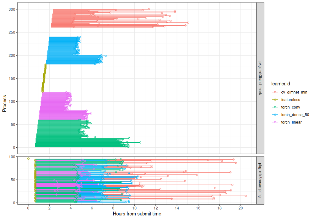
Above we can see the differences between the two parallelization methods more clearly.
Conclusions
We explored a method of parallelization via a lock file and a shared CSV. We saw that this method can more efficiently use cluster resources.
Session info
sessionInfo()
## R Under development (unstable) (2025-05-21 r88220)
## Platform: x86_64-pc-linux-gnu
## Running under: Ubuntu 24.04.2 LTS
##
## Matrix products: default
## BLAS:   /usr/lib/x86_64-linux-gnu/blas/libblas.so.3.12.0
## LAPACK: /usr/lib/x86_64-linux-gnu/lapack/liblapack.so.3.12.0  LAPACK version 3.12.0
##
## locale:
##  [1] LC_CTYPE=fr_FR.UTF-8       LC_NUMERIC=C               LC_TIME=fr_FR.UTF-8        LC_COLLATE=fr_FR.UTF-8
##  [5] LC_MONETARY=fr_FR.UTF-8    LC_MESSAGES=fr_FR.UTF-8    LC_PAPER=fr_FR.UTF-8       LC_NAME=C
##  [9] LC_ADDRESS=C               LC_TELEPHONE=C             LC_MEASUREMENT=fr_FR.UTF-8 LC_IDENTIFICATION=C
##
## time zone: Europe/Paris
## tzcode source: system (glibc)
##
## attached base packages:
## [1] stats     graphics  grDevices utils     datasets  methods   base
##
## other attached packages:
## [1] mlr3resampling_2025.6.23 mlr3_1.0.0.9000          future_1.58.0            ggplot2_3.5.1
## [5] data.table_1.17.99
##
## loaded via a namespace (and not attached):
##  [1] tidyselect_1.2.1       dust_0.3.0             dplyr_1.1.4            farver_2.1.2           filelock_1.0.3
##  [6] fastmap_1.2.0          promises_1.3.2         paradox_1.0.1          digest_0.6.37          rpart_4.1.24
## [11] base64url_1.4          mime_0.13              lifecycle_1.0.4        ellipsis_0.3.2         processx_3.8.6
## [16] magrittr_2.0.3         compiler_4.6.0         rlang_1.1.6            progress_1.2.3         tools_4.6.0
## [21] knitr_1.50             prettyunits_1.2.0      labeling_0.4.3         brew_1.0-10            htmlwidgets_1.6.4
## [26] pkgbuild_1.4.7         curl_6.2.2             plyr_1.8.9             batchtools_0.9.17      pkgload_1.4.0
## [31] miniUI_0.1.1.1         withr_3.0.2            purrr_1.0.4            mlr3misc_0.18.0        desc_1.4.3
## [36] grid_4.6.0             urlchecker_1.0.1       profvis_0.4.0          mlr3measures_1.0.0     xtable_1.8-4
## [41] colorspace_2.1-1       globals_0.18.0         scales_1.3.0           cli_3.6.5              crayon_1.5.3
## [46] generics_0.1.3         remotes_2.5.0          future.apply_1.20.0    directlabels_2025.5.20 sessioninfo_1.2.3
## [51] atime_2025.5.24        cachem_1.1.0           parallel_4.6.0         fpopw_1.2              vctrs_0.6.5
## [56] devtools_2.4.5         animint2_2025.6.4      callr_3.7.6            hms_1.1.3              listenv_0.9.1
## [61] lgr_0.4.4              glue_1.8.0             parallelly_1.45.0      RJSONIO_1.3-1.9        codetools_0.2-20
## [66] ps_1.9.1               stringi_1.8.7          gtable_0.3.6           later_1.4.1            quadprog_1.5-8
## [71] palmerpenguins_0.1.1   munsell_0.5.1          tibble_3.2.1           pillar_1.10.2          rappdirs_0.3.3
## [76] htmltools_0.5.8.1      R6_2.6.1               lattice_0.22-7         evaluate_1.0.3         shiny_1.10.0
## [81] backports_1.5.0        memoise_2.0.1          httpuv_1.6.15          Rcpp_1.0.14            uuid_1.2-1
## [86] checkmate_2.3.2        xfun_0.51              fs_1.6.6               usethis_3.1.0          pkgconfig_2.0.3