The goal of this post is to demonstrate that the performance of data.table CSV readers/writers is competitive with similar libraries available in Python (pandas, duckdb, polars). Compare with the previous post, which compared R functions (not python).

What is the overhead of communication with python from R?

We will be recording the timings of python code from R, via the reticulate package. To use that, we must tell reticulate where to find a python (conda environment) which has pandas installed:

reticulate::use_condaenv("~/miniconda3/envs/2023-08-deep-learning/bin/python3.11")

If you want to reproduce the results in this blog on your own computer, make sure to change the line above to a valid conda environment.

Below, we run a test to determine what is the overhead involved in communicating with python from R via reticulate.

atime.overhead <- atime::atime(
  N = as.integer(10^seq(0, 3, by = 0.5)),
  overhead = {
    reticulate::py_run_string("x = 5")
  }
)
atime.overhead$unit.col.vec <- c(seconds="median")
plot(atime.overhead)

plot of chunk overhead

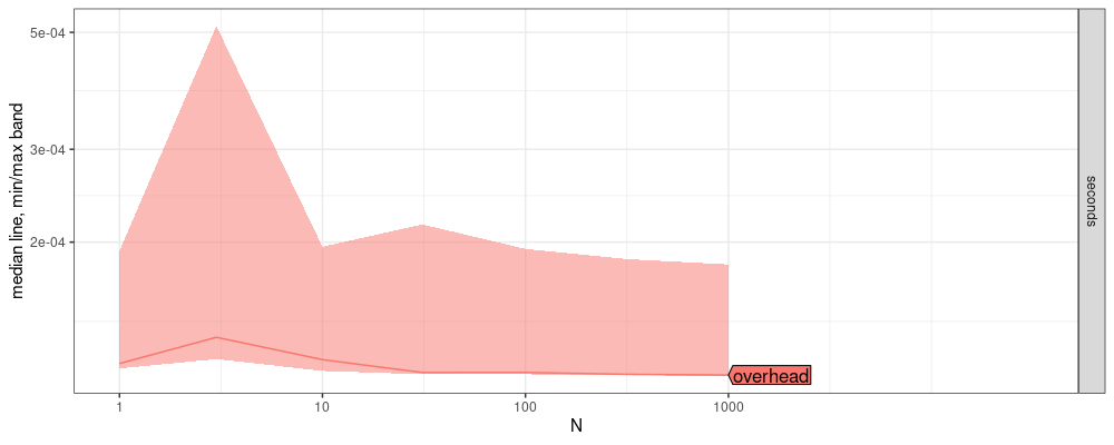
(overhead.seconds <- median(atime.overhead$measurements$median))

## [1] 0.0001131966

The plot above shows that the overhead of communication between R and python is about 0.1131966 milliseconds.

write csv, vary columns, char

This section compares the performance of CSV files with a variable number of character/string columns..

library(data.table)
reticulate::py_run_string("import pandas as pd")
N_rows <- 100
(N_col_seq <- unique(as.integer(10^seq(0, 6, by = 0.2))))

##  [1]       1       2       3       6      10      15      25      39      63     100     158     251     398     630
## [15]    1000    1584    2511    3981    6309   10000   15848   25118   39810   63095  100000  158489  251188  398107
## [29]  630957 1000000

main <- reticulate::py
con <- duckdb::dbConnect(duckdb::duckdb(), dbdir = ":memory:")
atime.write.chr.cols <- atime::atime(
  N = N_col_seq,
  setup = {
    input.chr <- matrix(c("foo", "x", "bar", NA), N_rows, N)
    input.df <- data.frame(input.chr)
    polars.df <- polars::as_polars_df(input.df)
    main$input_df_pd <- input.df
    input.dt <- data.table(input.df)
    duckdb::dbWriteTable(con, "duck_table", input.df, overwrite=TRUE)
    out.csv <- sprintf("%s/data_N=%d.csv", tempdir(), N)
  },
  seconds.limit = 0.1,
  "data.table\nfwrite" = {
    data.table::fwrite(input.dt, out.csv, showProgress = FALSE)
  },
  "pandas\nto_csv" = {
    reticulate::py_run_string("input_df_pd.to_csv('data.csv', index=False)")
  },
  "polars\nto_csv" = {
    polars.df$write_csv('polars.csv')
  },
  "duckdb\nCOPY" = { # https://duckdb.org/docs/guides/file_formats/csv_export.html
    DBI::dbSendQuery(con, "COPY duck_table TO 'duck.csv' (HEADER, DELIMITER ',')")
  }
)
atime.write.chr.cols$unit.col.vec <- c(seconds="median")
library(ggplot2)
plot(atime.write.chr.cols)+
  geom_hline(aes(
    yintercept=overhead.seconds),
    color="grey50",
    data=data.frame(overhead.seconds))

plot of chunk write-chr-cols

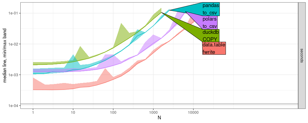
The plot above shows a colored curve for each CSV writing function. The grey horizontal line shows the overhead of communication with python from R. We see that the overhead (grey line) is insignificant, compared with the CSV writing timings (colored curves). The code below shows the throughput of each function at the specified time limit.

refs.write.chr.cols <- atime::references_best(atime.write.chr.cols)
pred.write.chr.cols <- predict(refs.write.chr.cols)
plot(pred.write.chr.cols)+
  ggtitle("Write strings to CSV, 100 x N")+
  scale_x_log10("N = number of columns to write")+
  scale_y_log10("Computation time (seconds)\nmedian line, min/max band\nover 10 timings",limits=c(1e-4,0.5))+
  facet_null()

## Scale for x is already present.
## Adding another scale for x, which will replace the existing scale.
## Scale for y is already present.
## Adding another scale for y, which will replace the existing scale.

## Warning in scale_x_log10("N = number of columns to write"): log-10 transformation introduced infinite values.

plot of chunk pred-write-chr-cols

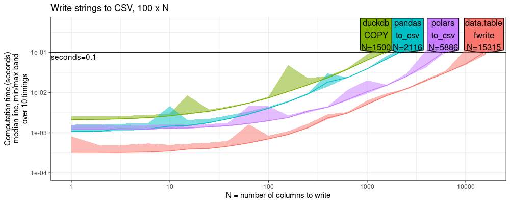
The plot above shows that data.table is competitive with the other libraries: about 2x faster than polars, and 10x faster than pandas/duckdb.

read CSV, vary columns, char

In this section we compare performance of CSV readers.

atime.read.chr.cols <- atime::atime(
  N = N_col_seq,
  setup = {
    in.csv <- sprintf("%s/data_N=%d.csv", tempdir(), N)
    pandas_cmd <- sprintf("pd.read_csv('%s')", in.csv)
    ## https://duckdb.org/docs/data/csv/overview.html
    duck_cmd <- sprintf("SELECT * FROM read_csv('%s', delim=',', header=true)", in.csv)
  },
  seconds.limit = 0.1,
  "data.table\nfread" = {
    data.table::fread(in.csv, showProgress = FALSE)
  },
  "pandas\nread_csv" = {
    reticulate::py_run_string(pandas_cmd)
  },
  "duckdb\nread_csv" = {
    DBI::dbSendQuery(con, duck_cmd)
  },
  "polars\nread_csv" = {
    polars::pl$read_csv(in.csv)
  }
)
refs.read.chr.cols <- atime::references_best(atime.read.chr.cols)
pred.read.chr.cols <- predict(refs.read.chr.cols)
plot(pred.read.chr.cols)+
  ggtitle("Read strings from CSV, 100 x N")+
  scale_x_log10("N = number of columns to read")+
  scale_y_log10("Computation time (seconds)\nmedian line, min/max band\nover 10 timings",limits=c(1e-4,0.5))+
  facet_null()

## Scale for x is already present.
## Adding another scale for x, which will replace the existing scale.
## Scale for y is already present.
## Adding another scale for y, which will replace the existing scale.

## Warning in scale_x_log10("N = number of columns to read"): log-10 transformation introduced infinite values.

plot of chunk read-chr-cols

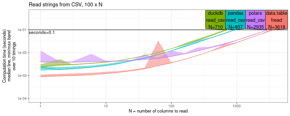
The plot above shows that data.table has the fastest CSV reader. The plot above shows the throughput at the time limit, which reveals that data.table is faster than polars by a small factor (less than 2x), but faster than duckdb/pandas by a larger amount (3-5x).

variants of these benchmarks

There are several variables we can play with in these benchmarks.

variable number of rows or columns (we did columns above)
numeric or character/string data (we did character/string above)
read or write (we did both above)

Below we consider two variants of the benchmark.

write csv, variable rows

Here we consider writing a variable number of rows (instead of cols above) for character/string data. (numeric data and reading are exercises for the reader)

atime.write.chr.rows <- atime::atime(
  setup = {
    input.chr <- matrix(c("foo", "x", "bar", NA), N, 10)
    input.df <- data.frame(input.chr)
    polars.df <- polars::as_polars_df(input.df)
    main$input_df_pd <- input.df
    input.dt <- data.table(input.df)
    duckdb::dbWriteTable(con, "duck_table", input.df, overwrite=TRUE)
    out.csv <- sprintf("%s/data_N=%d.csv", tempdir(), N)
  },
  seconds.limit = 0.01,
  "data.table\nfwrite" = {
    data.table::fwrite(input.dt, out.csv, showProgress = FALSE)
  },
  "pandas\nto_csv" = {
    reticulate::py_run_string("input_df_pd.to_csv('data.csv', index=False)")
  },
  "polars\nto_csv" = {
    polars.df$write_csv('polars.csv')
  },
  "duckdb\nCOPY" = { # https://duckdb.org/docs/guides/file_formats/csv_export.html
    DBI::dbSendQuery(con, "COPY duck_table TO 'duck.csv' (HEADER, DELIMITER ',')")
  }
)
refs.write.chr.rows <- atime::references_best(atime.write.chr.rows)
pred.write.chr.rows <- predict(refs.write.chr.rows)
plot(pred.write.chr.rows)+
  ggtitle("Write strings to CSV, N x 100")+
  scale_y_log10("Computation time (seconds)\nmedian line, min/max band\nover 10 timings")+
  facet_null()+
  scale_x_log10("N = number of rows to write")

## Scale for y is already present.
## Adding another scale for y, which will replace the existing scale.
## Scale for x is already present.
## Adding another scale for x, which will replace the existing scale.

## Warning in scale_x_log10("N = number of rows to write"): log-10 transformation introduced infinite values.

plot of chunk write-chr-rows

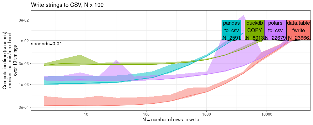
The plot above again shows that data.table is the fastest CSV writer. It is about the same as polars (within 2x), about 3x faster than duckdb, and 10x faster than pandas.

write csv, numeric cols

Here we consider writing a variable number of cols for numeric data (instead of character/string data above). Variable number of rows, and reading instead of writing, are exercises for the reader.

atime.write.num.cols <- atime::atime(
  N = N_col_seq,
  setup = {
    set.seed(1)
    input.num <- matrix(rnorm(N_rows * N), N_rows, N)
    input.num[sample(N_rows*N, N)] <- NA
    input.df <- data.frame(input.num)
    polars.df <- polars::as_polars_df(input.df)
    main$input_df_pd <- input.df
    input.dt <- data.table(input.df)
    duckdb::dbWriteTable(con, "duck_table", input.df, overwrite=TRUE)
    out.csv <- sprintf("%s/data_N=%d.csv", tempdir(), N)
  },
  seconds.limit = 0.1,
  "data.table\nfwrite" = {
    data.table::fwrite(input.dt, out.csv, showProgress = FALSE)
  },
  "pandas\nto_csv" = {
    reticulate::py_run_string("input_df_pd.to_csv('data.csv', index=False)")
  },
  "polars\nto_csv" = {
    polars.df$write_csv('polars.csv')
  },
  "duckdb\nCOPY" = { # https://duckdb.org/docs/guides/file_formats/csv_export.html
    DBI::dbSendQuery(con, "COPY duck_table TO 'duck.csv' (HEADER, DELIMITER ',')")
  }
)
refs.write.num.cols <- atime::references_best(atime.write.num.cols)
pred.write.num.cols <- predict(refs.write.num.cols)
plot(pred.write.num.cols)+
  ggtitle("Write real numbers to CSV, 100 x N")+
  scale_y_log10("Computation time (seconds)\nmedian line, min/max band\nover 10 timings",limits=c(1e-4,0.5))+
  facet_null()+
  scale_x_log10("N = number of columns to write")

## Scale for y is already present.
## Adding another scale for y, which will replace the existing scale.
## Scale for x is already present.
## Adding another scale for x, which will replace the existing scale.

## Warning in scale_x_log10("N = number of columns to write"): log-10 transformation introduced infinite values.

plot of chunk write-num-cols

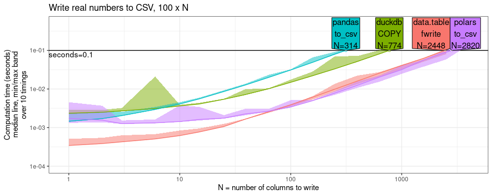
The code above shows the throughput of each function at the specified time limit. The plot above shows that data.table is competitive with the other libraries: almost as fast as polars, and several times faster than pandas/duckdb. This indicates that data.table is especially efficient for character/string data (rather than numeric data).

Summarize by group

In this section, we compare the time required for computing a summarization. In machine learning we often run gradient descent for several epochs, and we want to average the loss over cross-validation folds. The experiment below assumes we have 10 cross-validation folds, and N epochs.

n.folds <- 10
ml.atime <- atime::atime(
  setup={
    set.seed(1)
    loss.dt <- data.table(
      name="loss", 
      fold=rep(1:n.folds, each=N),
      loss=rnorm(N*n.folds),
      set=rep(c("subtrain","validation"),each=N/2),
      epoch=seq(1,N/2),
      key=c("set","epoch","fold"))
    loss.polars <- polars::as_polars_df(loss.dt)
    main$loss_df_pd <- loss.dt
    duckdb::dbWriteTable(con, "loss_table", loss.dt, overwrite=TRUE)
  },
  seconds.limit=0.1,
  data.table={
    loss.dt[, .(
      loss_length=.N,
      loss_mean=mean(loss),
      loss_sd=sd(loss)
    ), by=.(set, epoch)]
  },
  polars={
    loss.polars$group_by(c("set","epoch"))$agg(
      loss_len=polars::pl$col("loss")$len(),
      loss_mean=polars::pl$col("loss")$mean(),
      loss_std=polars::pl$col("loss")$std())
  },
  pandas={
    reticulate::py_run_string("loss_df_pd.groupby(['set','epoch']).loss.agg(['size','mean','std'])")
  },
  duckdb={
    DBI::dbSendQuery(con, "
SELECT set, epoch, 
count(*) as loss_count, 
mean(loss) as loss_mean, 
stddev(loss) as loss_stddev 
FROM loss_table 
GROUP BY set, epoch")
  })
ml.refs <- atime::references_best(ml.atime)
ml.pred <- predict(ml.refs)
plot(ml.pred)+
  ggtitle(sprintf("Mean,SD,Length over %d real numbers, N times", n.folds))+
  scale_x_log10("N = number of Mean,SD,Length to compute")+
  scale_y_log10("Computation time (seconds)\nmedian line, min/max band\nover 10 timings")+
  facet_null()

## Scale for x is already present.
## Adding another scale for x, which will replace the existing scale.
## Scale for y is already present.
## Adding another scale for y, which will replace the existing scale.

## Warning in scale_x_log10("N = number of Mean,SD,Length to compute"): log-10 transformation introduced infinite values.

plot of chunk summarize

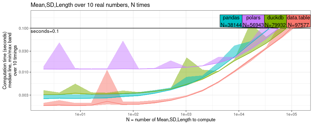
The result above shows that data.table is 2-3x faster than the other software.

Conclusions

We have shown that data.table can be faster than similar libraries which can be used from python or R.

Session info

sessionInfo()

## R Under development (unstable) (2024-10-01 r87205)
## Platform: x86_64-pc-linux-gnu
## Running under: Ubuntu 22.04.5 LTS
## 
## Matrix products: default
## BLAS:   /usr/lib/x86_64-linux-gnu/blas/libblas.so.3.10.0 
## LAPACK: /home/tdhock/miniconda3/envs/2023-08-deep-learning/lib/libmkl_rt.so.2;  LAPACK version 3.10.1
## 
## locale:
##  [1] LC_CTYPE=fr_FR.UTF-8       LC_NUMERIC=C               LC_TIME=fr_FR.UTF-8        LC_COLLATE=fr_FR.UTF-8    
##  [5] LC_MONETARY=fr_FR.UTF-8    LC_MESSAGES=fr_FR.UTF-8    LC_PAPER=fr_FR.UTF-8       LC_NAME=C                 
##  [9] LC_ADDRESS=C               LC_TELEPHONE=C             LC_MEASUREMENT=fr_FR.UTF-8 LC_IDENTIFICATION=C       
## 
## time zone: America/New_York
## tzcode source: system (glibc)
## 
## attached base packages:
## [1] stats     graphics  utils     datasets  grDevices methods   base     
## 
## other attached packages:
## [1] ggplot2_3.5.1     data.table_1.16.2
## 
## loaded via a namespace (and not attached):
##  [1] Matrix_1.7-0           gtable_0.3.4           jsonlite_1.8.8         dplyr_1.1.4            compiler_4.5.0        
##  [6] highr_0.11             tidyselect_1.2.1       Rcpp_1.0.12            scales_1.3.0           png_0.1-8             
## [11] directlabels_2024.1.21 reticulate_1.34.0.9000 lattice_0.22-6         R6_2.5.1               labeling_0.4.3        
## [16] generics_0.1.3         knitr_1.47             tibble_3.2.1           polars_0.19.1          munsell_0.5.0         
## [21] atime_2024.12.3        DBI_1.2.1              pillar_1.9.0           rlang_1.1.3            utf8_1.2.4            
## [26] xfun_0.45              quadprog_1.5-8         cli_3.6.2              withr_3.0.0            magrittr_2.0.3        
## [31] grid_4.5.0             lifecycle_1.0.4        vctrs_0.6.5            bench_1.1.3            evaluate_0.23         
## [36] glue_1.7.0             farver_2.1.1           duckdb_1.1.0           profmem_0.6.0          fansi_1.0.6           
## [41] colorspace_2.1-0       tools_4.5.0            pkgconfig_2.0.3

reticulate::py_run_string("print(pd.__version__)")

## 2.1.1