Cross-validation experiments with torch learners
The goal of this post is to show how to use the mlr3torch package in R with in combination with mlr3resampling, which contains the new cross-validation methods we proposed in our SOAK paper.
Introduction
Last Friday I gave a talk at MILA, Two new algorithms for scientific applications of machine learning. The first algorithm that I discussed is SOAK: Same/Other/All K-fold cross-validation for estimating similarity of patterns in data subsets. One simple demonstration of the algorithm involves three image classification benchmark data sets. Code below adapted from my github repo:
other.name.vec <- c("EMNIST", "FashionMNIST")
data.name.vec <- c(other.name.vec, "MNIST")
First we download those data sets.
prefix <- "https://rcdata.nau.edu/genomic-ml/cv-same-other-paper/data_Classif/"
data_Classif <- "~/projects/cv-same-other-paper/data_Classif"
options(timeout = 600)#seconds
for(data.name in data.name.vec){
  data.csv <- paste0(data.name, ".csv")
  local.csv <- file.path(data_Classif, data.csv)
  if(!file.exists(local.csv)){
    remote.csv <- paste0(prefix, data.csv)
    download.file(remote.csv, local.csv)
  }
}
Next we read these data into R (only the first few rows, for demonstration purposes).
data.list <- list()
library(data.table)
for(data.name in data.name.vec){
  data.csv <- paste0(data.name, ".csv")
  local.csv <- file.path(data_Classif, data.csv)
  data.list[[data.name]] <- fread(local.csv, nrows = 1000)
}
Next, we plot an example of each class. To do that in the ggplot framework, we need to create a data frame with one row per pixel to display, as in the code below.
n.pixels <- 28
pseq <- 1:n.pixels
(one.ex.dt <- data.table(Data=data.name.vec)[, {
  data.list[[Data]][, data.table(
    intensity=unlist(.SD[1]),
    pixel_j=rep(pseq, n.pixels),
    pixel_i=rep(pseq, each=n.pixels)
  ), by=y, .SDcols=patterns("[0-9]")]
}, by=Data])
##          Data     y intensity pixel_j pixel_i
##        <char> <int>     <num>   <int>   <int>
##     1: EMNIST     4         0       1       1
##     2: EMNIST     4         0       2       1
##     3: EMNIST     4         0       3       1
##     4: EMNIST     4         0       4       1
##     5: EMNIST     4         0       5       1
##    ---
## 23516:  MNIST     8         0      24      28
## 23517:  MNIST     8         0      25      28
## 23518:  MNIST     8         0      26      28
## 23519:  MNIST     8         0      27      28
## 23520:  MNIST     8         0      28      28
We can visualize the images by using the ggplot code below.
library(ggplot2)
ggplot()+
  theme_bw()+
  theme(panel.spacing=grid::unit(0,"lines"))+
  scale_y_reverse()+
  scale_fill_gradient(low="white",high="black")+
  geom_tile(aes(
    pixel_j, pixel_i, fill=intensity),
    data=one.ex.dt)+
  facet_grid(Data ~ y)+
  coord_equal()
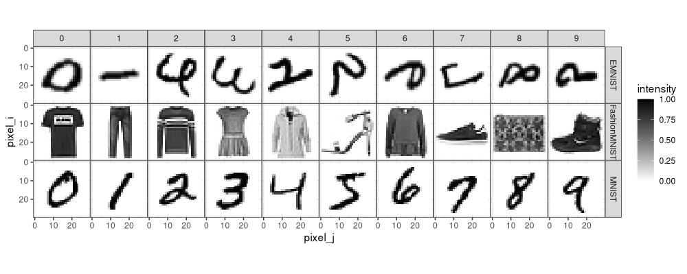
We see in the image above that the EMNIST digits are transposed (rotated 90 degrees and flipped) with respect to the MNIST digits. Correction below.
data.list$EMNIST_rot <- data.list$EMNIST[,c(
  1,2,as.integer(matrix(seq(1,n.pixels^2),n.pixels,n.pixels,byrow=TRUE))+2
),with=FALSE]
(one.ex.dt <- data.table(Data=names(data.list))[, {
  data.list[[Data]][, data.table(
    intensity=unlist(.SD[1]),
    pixel_j=rep(pseq, n.pixels),
    pixel_i=rep(pseq, each=n.pixels)
  ), by=y, .SDcols=patterns("[0-9]")]
}, by=Data])
##              Data     y intensity pixel_j pixel_i
##            <char> <int>     <num>   <int>   <int>
##     1:     EMNIST     4         0       1       1
##     2:     EMNIST     4         0       2       1
##     3:     EMNIST     4         0       3       1
##     4:     EMNIST     4         0       4       1
##     5:     EMNIST     4         0       5       1
##    ---
## 31356: EMNIST_rot     2         0      24      28
## 31357: EMNIST_rot     2         0      25      28
## 31358: EMNIST_rot     2         0      26      28
## 31359: EMNIST_rot     2         0      27      28
## 31360: EMNIST_rot     2         0      28      28
ggplot()+
  theme_bw()+
  theme(panel.spacing=grid::unit(0,"lines"))+
  scale_y_reverse()+
  scale_fill_gradient(low="white",high="black")+
  geom_tile(aes(
    pixel_j, pixel_i, fill=intensity),
    data=one.ex.dt)+
  facet_grid(Data ~ y)+
  coord_equal()
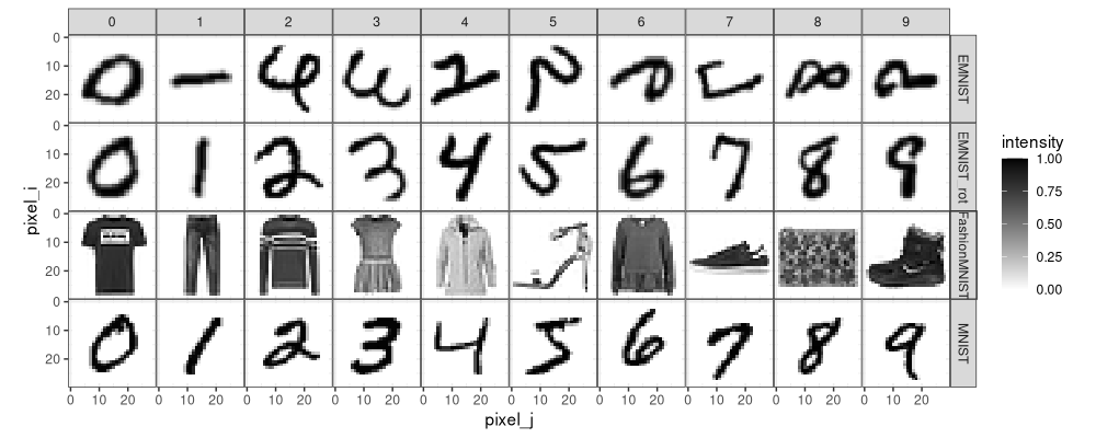
Above we see the EMNIST_rot data in the same orientation as the MNIST data.
Convert data to torch tensors
In my Res Baz 2023 tutorial, I explained how to use torch in R. The first step is to convert the data from R to a torch tensor.
ex.dt <- data.list$FashionMNIST
ex.X.mat <- as.matrix(ex.dt[,-(1:2),with=FALSE])
ex.X.array <- array(ex.X.mat, c(nrow(ex.dt), 1, n.pixels, n.pixels))
ex.X.tensor <- torch::torch_tensor(ex.X.array)
ex.X.tensor$shape
## [1] 1000 1 28 28
(ex.y.tensor <- torch::torch_tensor(ex.dt$y+1L, torch::torch_long()))
## torch_tensor
##  10
##   1
##   1
##   4
##   1
##   3
##   8
##   3
##   6
##   6
##   1
##  10
##   6
##   6
##   8
##  10
##   2
##   1
##   7
##   5
##   4
##   2
##   5
##   9
##   5
##   4
##   1
##   3
##   5
##   5
## ... [the output was truncated (use n=-1 to disable)]
## [ CPULongType{1000} ]
The data above represents a set of images in torch. Note that there are four dimensions used to represent the images:
- the first dimension represents the different images (
nrow(ex.dt)elements in the example above, one for each image). - the second dimension represents the color channels (1 in the example above, for grayscale images).
- the third and fourth dimensions represent the height and width of the image in pixels (28 in the example above).
torch linear model
A linear model is defined in the code below.
torch::torch_manual_seed(1)
n.features <- ncol(ex.X.mat)
n.classes <- 10
seq_linear_model <- torch::nn_sequential(
  torch::nn_flatten(),
  torch::nn_linear(n.features, n.classes))
two.X.tensor <- ex.X.tensor[1:2,,,]
(seq_linear_model_pred <- seq_linear_model(two.X.tensor))
## torch_tensor
## -0.1745  0.1314 -0.4476 -0.6590 -0.7359 -0.0889  0.6471  0.2814 -0.0880 -0.3649
##  0.1117  0.1763 -0.1807 -0.1092 -0.3902 -0.8008  0.3241  0.4483 -0.0729 -0.2066
## [ CPUFloatType{2,10} ][ grad_fn = <AddmmBackward0> ]
The prediction of the linear model is a tensor with two rows and ten columns (one output column for each class). To do learning we need to call backward on the result of a loss function, as in the code below.
seq_linear_model$parameters[[2]]$grad
## torch_tensor
## [ Tensor (undefined) ]
celoss <- torch::nn_cross_entropy_loss()
two.y.tensor <- ex.y.tensor[1:2]
(seq_linear_model_loss <- celoss(seq_linear_model_pred, two.y.tensor))
## torch_tensor
## 2.38987
## [ CPUFloatType{} ][ grad_fn = <NllLossBackward0> ]
seq_linear_model_loss$backward()
seq_linear_model$parameters[[2]]$grad
## torch_tensor
## -0.3985
##  0.1213
##  0.0764
##  0.0731
##  0.0599
##  0.0716
##  0.1720
##  0.1501
##  0.0960
## -0.4217
## [ CPUFloatType{10} ]
Note in the output above that grad is undefined at first, and then
defined after having called backward().
Learning with linear model
For learning we should first divide train data into subtrain and validation.
set_names <- c("validation", "subtrain")
set_vec <- rep(set_names, l=nrow(ex.dt))
table(set_vec, torch::as_array(ex.y.tensor))
##
## set_vec       1  2  3  4  5  6  7  8  9 10
##   subtrain   53 50 46 50 48 53 44 59 50 47
##   validation 54 54 40 42 47 47 56 56 52 52
The table above shows that there are about an equal number of observations in each class and set. Then we can use a gradient descent learning for loop,
n.epochs <- 1000
step_size <- 0.1
optimizer <- torch::optim_sgd(seq_linear_model$parameters, lr=step_size)
loss_dt_list <- list()
for(epoch in 1:n.epochs){
  set_loss_list <- list()
  for(set_name in set_names){
    is_set <- set_vec==set_name
    set_pred <- seq_linear_model(ex.X.tensor[is_set,,,])
    set_y <- ex.y.tensor[is_set]
    is_error <- set_y != set_pred$argmax(dim=2)
    N_errors <- torch::as_array(is_error$sum())
    batch_size <- length(set_y)
    set_loss_list[[set_name]] <- celoss(set_pred, set_y)
    loss_dt_list[[paste(epoch, set_name)]] <- data.table(
      epoch, set_name=factor(set_name, set_names),
      variable=c("error_percent","loss"),
      value=c(
        100*N_errors/length(is_error),
        torch::as_array(set_loss_list[[set_name]])))
  }
  optimizer$zero_grad()
  set_loss_list$subtrain$backward()
  optimizer$step()
}
(loss_dt <- rbindlist(loss_dt_list))
##       epoch   set_name      variable      value
##       <int>     <fctr>        <char>      <num>
##    1:     1 validation error_percent 93.8000000
##    2:     1 validation          loss  2.3194034
##    3:     1   subtrain error_percent 92.8000000
##    4:     1   subtrain          loss  2.3219512
##    5:     2 validation error_percent 65.0000000
##   ---
## 3996:   999   subtrain          loss  0.1862517
## 3997:  1000 validation error_percent 16.8000000
## 3998:  1000 validation          loss  0.5566300
## 3999:  1000   subtrain error_percent  2.0000000
## 4000:  1000   subtrain          loss  0.1861107
(min_dt <- loss_dt[, .SD[which.min(value)], by=.(variable,set_name)])
##         variable   set_name epoch      value
##           <char>     <fctr> <int>      <num>
## 1: error_percent validation   314 16.6000000
## 2:          loss validation   874  0.5560604
## 3: error_percent   subtrain   999  2.0000000
## 4:          loss   subtrain  1000  0.1861107
ggplot()+
  geom_line(aes(
    epoch, value, color=set_name),
    data=loss_dt)+
  geom_point(aes(
    epoch, value, color=set_name),
    shape=21,
    fill="white",
    data=min_dt)+
  facet_grid(variable ~ ., scales="free")
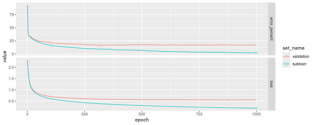
The results above show that the best validation error is about 16%, around 300 epochs. Notice how in the code above, we need for loops over epochs and sets, which is flexible but complicated.
Comparison with glmnet
Another implementation of linear models is given in the glmnet
package, which has automatic regularization parameter tuning via the
cv.glmnet function, but below we use the glmnet function for a
more direct comparison with what we did using torch above.
subtrain.X <- ex.X.mat[set_vec=="subtrain",]
ex.y.fac <- factor(torch::as_array(ex.y.tensor))
subtrain.y <- ex.y.fac[set_vec=="subtrain"]
fit_glmnet <- glmnet::glmnet(subtrain.X, subtrain.y, family="multinomial")
pred_glmnet <- predict(fit_glmnet, ex.X.mat, type="class")
err_glmnet_mat <- pred_glmnet != ex.y.fac

err_glmnet_dt_list <- list()
for(set_name in set_names){
  err_glmnet_dt_list[[set_name]] <- data.table(
    set_name=factor(set_name, set_names),
    penalty=fit_glmnet$lambda,
    complexity=-log10(fit_glmnet$lambda),
    error_percent=colMeans(err_glmnet_mat[set_vec==set_name,])*100)
}
err_glmnet_dt <- rbindlist(err_glmnet_dt_list)
(min_glmnet_dt <- err_glmnet_dt[, .SD[which.min(error_percent)], by=set_name])
##      set_name     penalty complexity error_percent
##        <fctr>       <num>      <num>         <num>
## 1: validation 0.003374554   2.471784          23.2
## 2:   subtrain 0.002325949   2.633400           0.0
ggplot()+
  theme_bw()+
  geom_line(aes(
    complexity, error_percent, color=set_name),
    data=err_glmnet_dt)+
  geom_point(aes(
    complexity, error_percent, color=set_name),
    data=min_glmnet_dt,
    shape=21,
    fill="white")+
  scale_x_log10(
    "Model complexity = -log10(L1 regularization parameter lambda)")
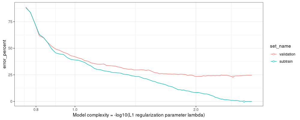
The figure above shows that the min validation error is about 23%, slightly larger than the torch linear model.
mlr3torch linear models
The mlr3torch package provides an alternative way of defining torch
models, using the
pipeops
framework. The advantage of this approach is that each model can be
converted to a Learner object, which can be run alongside other
non-torch learners (such as glmnet), on lots of different data sets
and train/test splits (in parallel using mlr3batchmark). They can be
even run using my newly proposed SOAK algorithm (Same/Other/All K-fold
cross-validation), which can be implemented using the code below.
soak <- mlr3resampling::ResamplingSameOtherSizesCV$new()
Note that it is important to run the line of code above, before
creating the tasks using the code below, because mlr3resampling
package needs to be loaded in order to avoid an error (subset is not
a valid column role).
The code below converts each data set of interest to a Task.
task.list <- list()
for(other.name in c("EMNIST_rot","FashionMNIST")){
  ipair.dt.list <- list()
  for(Data in c(other.name,"MNIST")){
    one.dt <- data.list[[Data]][,-1][, y := factor(y)][]
    setnames(one.dt, c("y", paste0("X", names(one.dt)[-1])))
    ipair.dt.list[[Data]] <- data.table(Data, one.dt)
  }
  ipair.dt <- rbindlist(ipair.dt.list, use.names=FALSE)
  ipair.name <- paste0("MNIST_",other.name)
  itask <- mlr3::TaskClassif$new(
    ipair.name, ipair.dt, target="y")
  itask$col_roles$stratum <- "y"
  itask$col_roles$subset <- "Data"
  itask$col_roles$feature <- paste0("X",seq(0,n.pixels^2-1))
  task.list[[ipair.name]] <- itask
}
task.list
## $MNIST_EMNIST_rot
## <TaskClassif:MNIST_EMNIST_rot> (2000 x 785)
## * Target: y
## * Properties: multiclass, strata
## * Features (784):
##   - dbl (784): X0, X1, X10, X100, X101, X102, X103, X104, X105, X106, X107, X108, X109, X11, X110, X111,
##     X112, X113, X114, X115, X116, X117, X118, X119, X12, X120, X121, X122, X123, X124, X125, X126, X127,
##     X128, X129, X13, X130, X131, X132, X133, X134, X135, X136, X137, X138, X139, X14, X140, X141, X142,
##     X143, X144, X145, X146, X147, X148, X149, X15, X150, X151, X152, X153, X154, X155, X156, X157, X158,
##     X159, X16, X160, X161, X162, X163, X164, X165, X166, X167, X168, X169, X17, X170, X171, X172, X173,
##     X174, X175, X176, X177, X178, X179, X18, X180, X181, X182, X183, X184, X185, X186, X187, X188, [...]
## * Strata: y
##
## $MNIST_FashionMNIST
## <TaskClassif:MNIST_FashionMNIST> (2000 x 785)
## * Target: y
## * Properties: multiclass, strata
## * Features (784):
##   - dbl (784): X0, X1, X10, X100, X101, X102, X103, X104, X105, X106, X107, X108, X109, X11, X110, X111,
##     X112, X113, X114, X115, X116, X117, X118, X119, X12, X120, X121, X122, X123, X124, X125, X126, X127,
##     X128, X129, X13, X130, X131, X132, X133, X134, X135, X136, X137, X138, X139, X14, X140, X141, X142,
##     X143, X144, X145, X146, X147, X148, X149, X15, X150, X151, X152, X153, X154, X155, X156, X157, X158,
##     X159, X16, X160, X161, X162, X163, X164, X165, X166, X167, X168, X169, X17, X170, X171, X172, X173,
##     X174, X175, X176, X177, X178, X179, X18, X180, X181, X182, X183, X184, X185, X186, X187, X188, [...]
## * Strata: y
Note that the code above produces a list of two tasks, each of which has two subsets.
MNIST_FashionMNISThas two subsets: half MNIST images (digits), half FashionMNIST images (clothing). It should not be possible to get good accuracy when training on MNIST and predicting on FashionMNIST.MNIST_EMNIST_rothas two subsets: half MNIST images (digits), half EMNIST images (also digits), so it may be possible to get good prediction, even though the two data sets have different pre-processing methods (slightly different position / size of digit images).
Define linear model using mlr3 MLP learner
To define a torch linear model in the mlr3 framework,
@sebffischer
advised me to first define a MLP, designating the number of epochs to
tune, with patience equal to the number of total epochs (meaning it
will always go up to the total number of epochs). Docs for this are in
mlr3 book chapter
15,
which explains about internal tuning via parameters like
early_stopping_rounds and patience.
measure_list <- mlr3::msrs(c("classif.logloss", "classif.ce"))
(mlp_learner = mlr3::lrn("classif.mlp",
  epochs = paradox::to_tune(upper = n.epochs, internal = TRUE),
  measures_train = measure_list,
  measures_valid = measure_list,
  patience = n.epochs,
  optimizer = mlr3torch::t_opt("sgd", lr = step_size),
  callbacks = mlr3torch::t_clbk("history"),
  batch_size = batch_size,
  validate = 0.5,
  predict_type = "prob"))
## <LearnerTorchMLP[classif]:classif.mlp>: My Little Powny
## * Model: -
## * Parameters: epochs=<InternalTuneToken>, device=auto, num_threads=1, num_interop_threads=1, seed=random,
##   jit_trace=FALSE, eval_freq=1, measures_train=<list>, measures_valid=<list>, patience=1000, min_delta=0,
##   batch_size=500, shuffle=TRUE, tensor_dataset=FALSE, neurons=integer(0), p=0.5, activation=<nn_relu>,
##   activation_args=<list>, opt.lr=0.1
## * Validate: 0.5
## * Packages: mlr3, mlr3torch, torch
## * Predict Types:  response, [prob]
## * Feature Types: integer, numeric, lazy_tensor
## * Properties: internal_tuning, marshal, multiclass, twoclass, validation
## * Optimizer: sgd
## * Loss: cross_entropy
## * Callbacks: history
Note in the output above that
neurons=integer(0), meaning there are no hidden units, implying a linear model.epochs=<InternalTuneToken>, meaning that the number of epochs is to be tuned using a held-out validation set (as is defined in the code below).
Below we create an auto tuner learner based on the MLP learner, instructing it to use the (first) internal validation score as the measure to optimize.
mlp_learner_auto = mlr3tuning::auto_tuner(
  learner = mlp_learner,
  tuner = mlr3tuning::tnr("internal"),
  resampling = mlr3::rsmp("insample"),# the train/valid split is handled by the learner itself
  measure = mlr3::msr("internal_valid_score", minimize = TRUE),# for the optimal model we will use the internal validation score computed during training
  term_evals = 1,# early stopping just needs a single run
  id="linear_mlp",
  store_models = TRUE)# so we can access the history afterwards
mlp_learner_auto$train(task.list$MNIST_FashionMNIST)
## INFO  [10:14:48.077] [bbotk] Starting to optimize 0 parameter(s) with '<TunerBatchInternal>' and '<TerminatorEvals> [n_evals=1, k=0]'
## INFO  [10:14:48.078] [bbotk] Evaluating 1 configuration(s)
## INFO  [10:14:48.083] [mlr3] Running benchmark with 1 resampling iterations
## INFO  [10:14:48.086] [mlr3] Applying learner 'classif.mlp' on task 'MNIST_FashionMNIST' (iter 1/1)
## INFO  [10:15:35.781] [mlr3] Finished benchmark
## INFO  [10:15:35.836] [bbotk] Result of batch 1:
## INFO  [10:15:35.837] [bbotk]  internal_valid_score warnings errors runtime_learners internal_tuned_values                                uhash
## INFO  [10:15:35.837] [bbotk]             0.7053771        0      0           47.527             <list[1]> ca34c414-9812-4b47-95b1-c6c013b3ba4d
## INFO  [10:15:35.858] [bbotk] Finished optimizing after 1 evaluation(s)
## INFO  [10:15:35.858] [bbotk] Result:
## INFO  [10:15:35.859] [bbotk]  internal_tuned_values learner_param_vals  x_domain internal_valid_score
## INFO  [10:15:35.859] [bbotk]                 <list>             <list>    <list>                <num>
## INFO  [10:15:35.859] [bbotk]              <list[1]>         <list[19]> <list[0]>            0.7053771
Note how simple this code is, relative to the code in the previous section, with a for loop over epochs. The advantage of mlr3torch is that typical models and training scenarios are greatly simplified – some flexibility is sacrificed, but we do not need that flexibility here to implement the linear model. The code below checks that the learned model is indeed a linear model:
mlp_learner_auto$model$learner$model$network
## An `nn_module` containing 7,850 parameters.
##
## ── Modules ────────────────────────────────────────────────────────────────────────────────
## • 0: <nn_linear> #7,850 parameters
We see that the number of parameters is consistent with a linear model
for 28*28=784 input features, and 10 outputs/classes.
Below we reshape and plot the epoch-specific measures which were used
to select the best number of epochs:
pat <- function(...){
  old2new <- c(...)
  if(is.null(names(old2new))){
    names(old2new) <- old2new
  }
  to.rep <- names(old2new)==""
  names(old2new)[to.rep] <- old2new[to.rep]
  list(
    paste(names(old2new), collapse="|"),
    function(x)factor(old2new[x], old2new))
}
melt_history <- function(DT)nc::capture_melt_single(
  DT,
  set=pat(valid="validation", train="subtrain"),
  ".classif.",
  measure=pat(ce="error_prop", auc="AUC", "logloss"))
(measure_long <- melt_history(
  mlp_learner_auto$archive$learners(1)[[1L]]$model$callbacks$history))
##       epoch        set    measure     value
##       <num>     <fctr>     <fctr>     <num>
##    1:     1   subtrain    logloss 2.2964028
##    2:     2   subtrain    logloss 2.1236063
##    3:     3   subtrain    logloss 1.9988996
##    4:     4   subtrain    logloss 1.8959093
##    5:     5   subtrain    logloss 1.8045186
##   ---
## 3996:   996 validation error_prop 0.2227772
## 3997:   997 validation error_prop 0.2227772
## 3998:   998 validation error_prop 0.2227772
## 3999:   999 validation error_prop 0.2217782
## 4000:  1000 validation error_prop 0.2227772
(selected_row <- as.data.table(
  mlp_learner_auto$tuning_result$internal_tuned_values[[1]]))
##    epochs
##     <int>
## 1:    532
ggplot()+
  facet_grid(measure ~ ., scales="free")+
  geom_vline(aes(
    xintercept=epochs),
    data=selected_row)+
  geom_line(aes(
    epoch, value, color=set),
    data=measure_long)
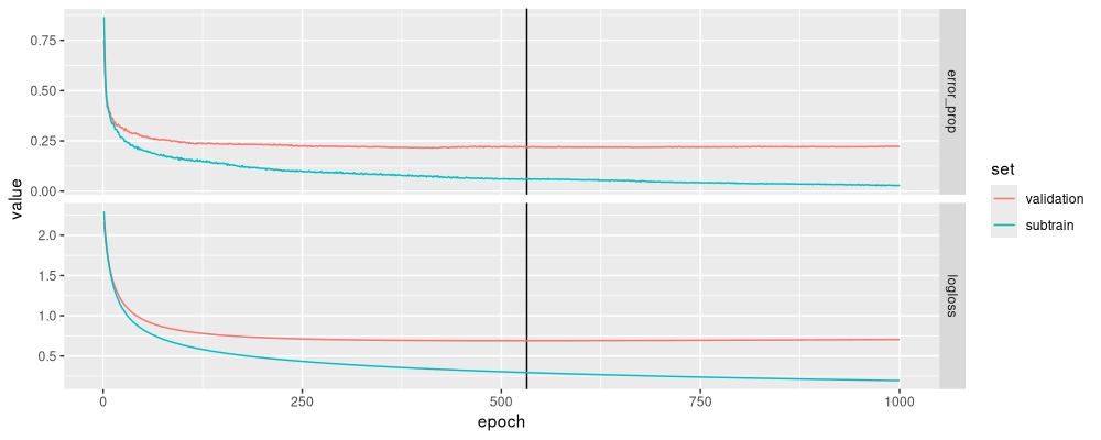
The figure above has learning curves that look reasonable.
Define mlr3 linear model using pipe operations
A more flexible way of defining a neural network involves pipe operations, as explained in mlr3torch-course-ch6, which explains how to mlr3torch pipe operations to define a neural network. Actually, this flexibility is not needed to define a linear model, but it would be if we wanted to define a more complex neural network (for example with convolutional layers), which will be the topic for a future blog.
I understand from ?mlr3torch::PipeOpTorchIngressNumeric
that we need po("torch_ingress_num") to convert regular R features
to torch tensors. And we need nn_head pipeop at the end of the
network, which automatically determines the right number of output
units, based on the loss function. Whereas the mlr3 docs suggest using
%>>% to combine pipe operations, I use list/Reduce below, to
emphasize which functions are defined in which packages.
po_list_linear_ce <- list(
  mlr3pipelines::po(
    "select",
    selector = mlr3pipelines::selector_type(c("numeric", "integer"))),
  mlr3torch::PipeOpTorchIngressNumeric$new(),
  mlr3pipelines::po("nn_head"),
  mlr3pipelines::po(
    "torch_loss",
    mlr3torch::t_loss("cross_entropy")),
  mlr3pipelines::po(
    "torch_optimizer",
    mlr3torch::t_opt("sgd", lr=step_size)),
  mlr3pipelines::po(
    "torch_callbacks",
    mlr3torch::t_clbk("history")),
  mlr3pipelines::po(
    "torch_model_classif",
    batch_size = batch_size,
    patience=n.epochs,
    measures_valid=measure_list,
    measures_train=measure_list,
    predict_type="prob",
    epochs = paradox::to_tune(upper = n.epochs, internal = TRUE)))
(graph_linear_ce <- Reduce(mlr3pipelines::concat_graphs, po_list_linear_ce))
## Graph with 7 PipeOps:
##                   ID         State            sccssors         prdcssors
##               <char>        <char>              <char>            <char>
##               select <<UNTRAINED>>   torch_ingress_num
##    torch_ingress_num <<UNTRAINED>>             nn_head            select
##              nn_head <<UNTRAINED>>          torch_loss torch_ingress_num
##           torch_loss <<UNTRAINED>>     torch_optimizer           nn_head
##      torch_optimizer <<UNTRAINED>>     torch_callbacks        torch_loss
##      torch_callbacks <<UNTRAINED>> torch_model_classif   torch_optimizer
##  torch_model_classif <<UNTRAINED>>                       torch_callbacks
Code above defines the graph learner object, and code below converts
it to a learner object. Note the set_validate is important to use
with pipe operations, to avoid some errors.
(glearner_linear_ce <- mlr3::as_learner(graph_linear_ce))
## <GraphLearner:select.torch_ingress_num.nn_head.torch_loss.torch_optimizer.torch_callbacks.torch_model_classif>
## * Model: -
## * Parameters: select.selector=<Selector>, torch_optimizer.lr=0.1,
##   torch_model_classif.epochs=<InternalTuneToken>, torch_model_classif.device=auto,
##   torch_model_classif.num_threads=1, torch_model_classif.num_interop_threads=1,
##   torch_model_classif.seed=random, torch_model_classif.jit_trace=FALSE, torch_model_classif.eval_freq=1,
##   torch_model_classif.measures_train=<list>, torch_model_classif.measures_valid=<list>,
##   torch_model_classif.patience=1000, torch_model_classif.min_delta=0, torch_model_classif.batch_size=500,
##   torch_model_classif.shuffle=TRUE, torch_model_classif.tensor_dataset=FALSE
## * Validate: NULL
## * Packages: mlr3, mlr3pipelines, mlr3torch, torch
## * Predict Types:  response, [prob]
## * Feature Types: logical, integer, numeric, character, factor, ordered, POSIXct, Date, lazy_tensor
## * Properties: featureless, hotstart_backward, hotstart_forward, importance, internal_tuning, marshal,
##   missings, multiclass, offset, oob_error, selected_features, twoclass, validation, weights
mlr3::set_validate(glearner_linear_ce, validate = 0.5)
The code below defines an auto tuner based on the graph learner above. It is the same as the corresponding code in the previous section with the MLP.
glearner_auto = mlr3tuning::auto_tuner(
  learner = glearner_linear_ce,
  tuner = mlr3tuning::tnr("internal"),
  resampling = mlr3::rsmp("insample"),
  measure = mlr3::msr("internal_valid_score", minimize = TRUE),
  term_evals = 1,
  id="linear_graph",
  store_models = TRUE)
glearner_auto$train(task.list$MNIST_FashionMNIST)
## INFO  [10:16:01.979] [bbotk] Starting to optimize 0 parameter(s) with '<TunerBatchInternal>' and '<TerminatorEvals> [n_evals=1, k=0]'
## INFO  [10:16:01.980] [bbotk] Evaluating 1 configuration(s)
## INFO  [10:16:01.984] [mlr3] Running benchmark with 1 resampling iterations
## INFO  [10:16:01.988] [mlr3] Applying learner 'select.torch_ingress_num.nn_head.torch_loss.torch_optimizer.torch_callbacks.torch_model_classif' on task 'MNIST_FashionMNIST' (iter 1/1)
## INFO  [10:17:44.845] [mlr3] Finished benchmark
## INFO  [10:17:44.906] [bbotk] Result of batch 1:
## INFO  [10:17:44.908] [bbotk]  internal_valid_score warnings errors runtime_learners internal_tuned_values                                uhash
## INFO  [10:17:44.908] [bbotk]             0.7314025        0      0          102.712             <list[1]> e2cc2233-7bf9-4e4f-a4f4-f864573d0788
## INFO  [10:17:44.943] [bbotk] Finished optimizing after 1 evaluation(s)
## INFO  [10:17:44.943] [bbotk] Result:
## INFO  [10:17:44.944] [bbotk]  internal_tuned_values learner_param_vals  x_domain internal_valid_score
## INFO  [10:17:44.944] [bbotk]                 <list>             <list>    <list>                <num>
## INFO  [10:17:44.944] [bbotk]              <list[1]>         <list[16]> <list[0]>            0.7314025
glearner_auto$base_learner()$model$network
## An `nn_module` containing 7,850 parameters.
##
## ── Modules ────────────────────────────────────────────────────────────────────────────────
## • module_list: <nn_module_list> #7,850 parameters
After training above, we visualize the model training below.
glearner_model <- glearner_auto$archive$learners(1)[[1]]$model
(glearner_long <- melt_history(
  glearner_model$torch_model_classif$model$callbacks$history))
##       epoch        set    measure     value
##       <num>     <fctr>     <fctr>     <num>
##    1:     1   subtrain    logloss 2.2776291
##    2:     2   subtrain    logloss 2.1146995
##    3:     3   subtrain    logloss 1.9905747
##    4:     4   subtrain    logloss 1.8862677
##    5:     5   subtrain    logloss 1.7931673
##   ---
## 3996:   996 validation error_prop 0.2187812
## 3997:   997 validation error_prop 0.2197802
## 3998:   998 validation error_prop 0.2187812
## 3999:   999 validation error_prop 0.2207792
## 4000:  1000 validation error_prop 0.2187812
(glearner_selected <- as.data.table(
  glearner_auto$tuning_result$internal_tuned_values[[1]]))
##    torch_model_classif.epochs
##                         <int>
## 1:                        453
ggplot()+
  facet_grid(measure ~ ., scales="free")+
  geom_vline(aes(
    xintercept=torch_model_classif.epochs),
    data=glearner_selected)+
  geom_line(aes(
    epoch, value, color=set),
    data=glearner_long)
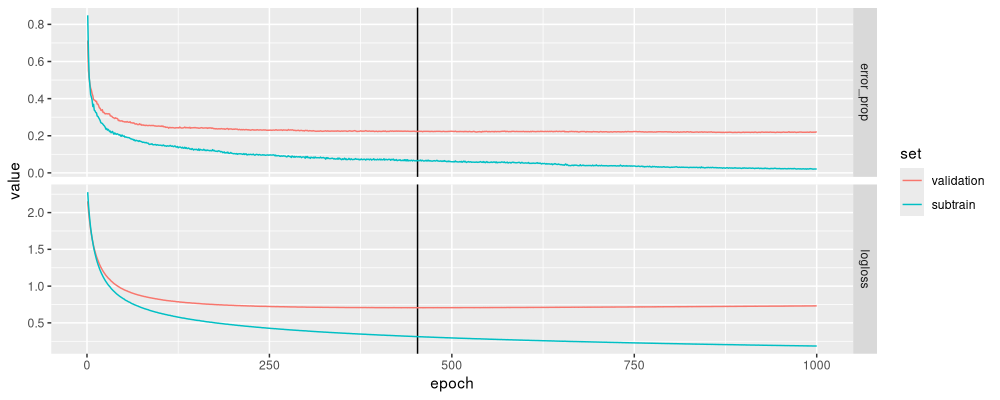
Again the plot looks reasonable, and consistent with our previous results.
Benchmark experiment
Is the torch linear model as accurate as the glmnet linear model?
Let’s find out. First we create a grid of learners and tasks. Note
that we add two learners based on glmnet, so we can see if
prediction error rates are affected by the choice of regularization
parameter (min validation loss or simplest model within 1se of min).
learner.list <- list(
  glearner_auto,
  mlp_learner_auto,
  mlr3::LearnerClassifFeatureless$new()$configure(id="featureless"))
for(s_param in c("min", "1se")){
  learner.list[[s_param]] <- mlr3learners::LearnerClassifCVGlmnet$new()$configure(
    s=paste0("lambda.",s_param),
    id=paste0("cv_glmnet_",s_param))
}
(bench.grid <- mlr3::benchmark_grid(
  task.list,
  learner.list,
  soak))
##                   task       learner          resampling
##                 <char>        <char>              <char>
##  1:   MNIST_EMNIST_rot  linear_graph same_other_sizes_cv
##  2:   MNIST_EMNIST_rot    linear_mlp same_other_sizes_cv
##  3:   MNIST_EMNIST_rot   featureless same_other_sizes_cv
##  4:   MNIST_EMNIST_rot cv_glmnet_min same_other_sizes_cv
##  5:   MNIST_EMNIST_rot cv_glmnet_1se same_other_sizes_cv
##  6: MNIST_FashionMNIST  linear_graph same_other_sizes_cv
##  7: MNIST_FashionMNIST    linear_mlp same_other_sizes_cv
##  8: MNIST_FashionMNIST   featureless same_other_sizes_cv
##  9: MNIST_FashionMNIST cv_glmnet_min same_other_sizes_cv
## 10: MNIST_FashionMNIST cv_glmnet_1se same_other_sizes_cv
Above we see a summary of the benchmark: two tasks, five learners, and
one resampling method. Below we declare a future plan for computation
in parallel on this machine. For larger experiments you can use
mlr3batchmark to compute in parallel on a cluster, see my blogs on
the importance of hyper-parameter
tuning
and Mammouth
tutorial. However
note that as of this writing, I have not got torch in R to work on
Mammouth (Sherbrooke’s super-computer), but a similar setup should
work on Beluga (another Alliance Canada super-computer where I have
got torch in R to work). Then we run/cache the benchmark:
cache.RData <- "2024-10-30-mlr3torch-benchmark.RData"
if(file.exists(cache.RData)){
  load(cache.RData)
}else{#code below should be run interactively.
  if(on.cluster){
    reg.dir <- "2024-10-30-mlr3torch-benchmark"
    unlink(reg.dir, recursive=TRUE)
    reg = batchtools::makeExperimentRegistry(
      file.dir = reg.dir,
      seed = 1,
      packages = "mlr3verse"
    )
    mlr3batchmark::batchmark(
      bench.grid, store_models = TRUE, reg=reg)
    job.table <- batchtools::getJobTable(reg=reg)
    chunks <- data.frame(job.table, chunk=1)
    batchtools::submitJobs(chunks, resources=list(
      walltime = 60*60,#seconds
      memory = 2000,#megabytes per cpu
      ncpus=1,  #>1 for multicore/parallel jobs.
      ntasks=1, #>1 for MPI jobs.
      chunks.as.arrayjobs=TRUE), reg=reg)
    batchtools::getStatus(reg=reg)
    jobs.after <- batchtools::getJobTable(reg=reg)
    table(jobs.after$error)
    ids <- jobs.after[is.na(error), job.id]
    bench.result <- mlr3batchmark::reduceResultsBatchmark(ids, reg = reg)
  }else{
    ## In the code below, we declare a multisession future plan to
    ## compute each benchmark iteration in parallel on this computer
    ## (data set, learning algorithm, cross-validation fold). For a
    ## few dozen iterations, using the multisession backend is
    ## probably sufficient (I have 12 CPUs on my work PC).
    if(require(future))plan("multisession")
    bench.result <- mlr3::benchmark(bench.grid, store_models = TRUE)
  }
  save(bench.result, file=cache.RData)
}
Then we compute and plot a table of evaluation metrics:
score_dt <- mlr3resampling::score(bench.result)[
, percent_error := 100*classif.ce
][]
score_dt[, .(task_id, test.subset, train.subsets, algorithm, percent_error)]
##                 task_id  test.subset train.subsets     algorithm percent_error
##                  <char>       <char>        <char>        <char>         <num>
##   1:   MNIST_EMNIST_rot   EMNIST_rot           all  linear_graph      16.71827
##   2:   MNIST_EMNIST_rot        MNIST           all  linear_graph      13.50575
##   3:   MNIST_EMNIST_rot   EMNIST_rot           all  linear_graph      16.09195
##   4:   MNIST_EMNIST_rot        MNIST           all  linear_graph      12.61830
##   5:   MNIST_EMNIST_rot   EMNIST_rot           all  linear_graph      12.46201
##  ---
## 176: MNIST_FashionMNIST        MNIST          same cv_glmnet_1se      15.10574
## 177: MNIST_FashionMNIST FashionMNIST          same cv_glmnet_1se      25.07463
## 178: MNIST_FashionMNIST        MNIST          same cv_glmnet_1se      18.37349
## 179: MNIST_FashionMNIST FashionMNIST          same cv_glmnet_1se      21.47239
## 180: MNIST_FashionMNIST        MNIST          same cv_glmnet_1se      19.58457
ggplot()+
  geom_point(aes(
    percent_error, algorithm),
    shape=1,
    data=score_dt)+
  facet_grid(train.subsets ~ task_id + test.subset, labeller=label_both)
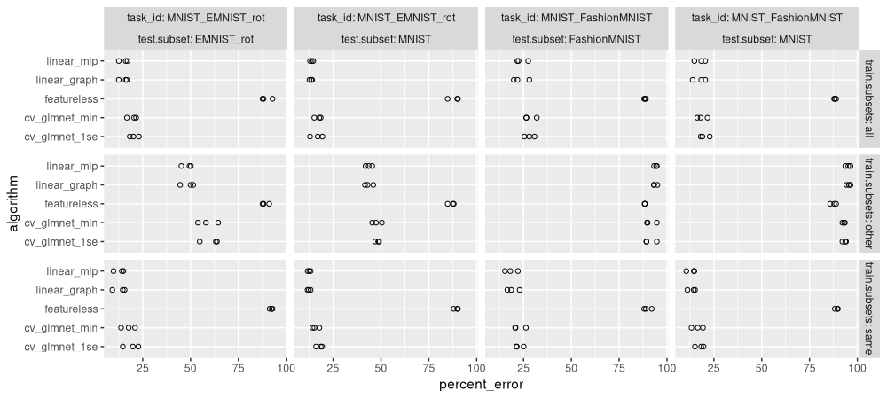
There is a lot of information in the plot above. It could be simplified by taking the mean and SD over the three folds:
(score_stats <- dcast(
  score_dt,
  algorithm + task_id + test.subset + train.subsets ~ .,
  list(mean, sd),
  value.var="percent_error"))
## Key: <algorithm, task_id, test.subset, train.subsets>
##         algorithm            task_id  test.subset train.subsets percent_error_mean percent_error_sd
##            <char>             <char>       <char>        <char>              <num>            <num>
##  1: cv_glmnet_1se   MNIST_EMNIST_rot   EMNIST_rot           all           20.44981        2.3924253
##  2: cv_glmnet_1se   MNIST_EMNIST_rot   EMNIST_rot         other           60.60458        5.0360943
##  3: cv_glmnet_1se   MNIST_EMNIST_rot   EMNIST_rot          same           19.03502        4.1115001
##  4: cv_glmnet_1se   MNIST_EMNIST_rot        MNIST           all           16.43025        3.2662652
##  5: cv_glmnet_1se   MNIST_EMNIST_rot        MNIST         other           48.17387        1.0326376
##  6: cv_glmnet_1se   MNIST_EMNIST_rot        MNIST          same           17.94955        1.6543981
##  7: cv_glmnet_1se MNIST_FashionMNIST FashionMNIST           all           28.07666        2.6434725
##  8: cv_glmnet_1se MNIST_FashionMNIST FashionMNIST         other           91.06927        3.1358809
##  9: cv_glmnet_1se MNIST_FashionMNIST FashionMNIST          same           22.59532        2.1503140
## 10: cv_glmnet_1se MNIST_FashionMNIST        MNIST           all           19.98382        2.5170842
## 11: cv_glmnet_1se MNIST_FashionMNIST        MNIST         other           93.29652        0.9979881
## 12: cv_glmnet_1se MNIST_FashionMNIST        MNIST          same           17.68793        2.3167806
## 13: cv_glmnet_min   MNIST_EMNIST_rot   EMNIST_rot           all           19.56750        2.5308583
## 14: cv_glmnet_min   MNIST_EMNIST_rot   EMNIST_rot         other           58.78455        5.3224331
## 15: cv_glmnet_min   MNIST_EMNIST_rot   EMNIST_rot          same           17.43396        3.6542630
## 16: cv_glmnet_min   MNIST_EMNIST_rot        MNIST           all           17.15517        1.7774342
## 17: cv_glmnet_min   MNIST_EMNIST_rot        MNIST         other           47.76247        2.5290389
## 18: cv_glmnet_min   MNIST_EMNIST_rot        MNIST          same           15.74519        1.8657007
## 19: cv_glmnet_min MNIST_FashionMNIST FashionMNIST           all           28.28978        3.1625618
## 20: cv_glmnet_min MNIST_FashionMNIST FashionMNIST         other           91.37327        2.8771981
## 21: cv_glmnet_min MNIST_FashionMNIST FashionMNIST          same           22.59217        3.1856577
## 22: cv_glmnet_min MNIST_FashionMNIST        MNIST           all           18.68274        2.7255241
## 23: cv_glmnet_min MNIST_FashionMNIST        MNIST         other           92.89637        0.6806662
## 24: cv_glmnet_min MNIST_FashionMNIST        MNIST          same           16.38238        3.0016185
## 25:   featureless   MNIST_EMNIST_rot   EMNIST_rot           all           89.52603        2.8615653
## 26:   featureless   MNIST_EMNIST_rot   EMNIST_rot         other           88.95132        1.8726767
## 27:   featureless   MNIST_EMNIST_rot   EMNIST_rot          same           92.18286        0.7661164
## 28:   featureless   MNIST_EMNIST_rot        MNIST           all           88.31289        2.9979853
## 29:   featureless   MNIST_EMNIST_rot        MNIST         other           86.85381        1.7408543
## 30:   featureless   MNIST_EMNIST_rot        MNIST          same           89.36442        1.1859407
## 31:   featureless MNIST_FashionMNIST FashionMNIST           all           88.50411        0.4487377
## 32:   featureless MNIST_FashionMNIST FashionMNIST         other           88.39911        0.0838583
## 33:   featureless MNIST_FashionMNIST FashionMNIST          same           89.68405        2.0851700
## 34:   featureless MNIST_FashionMNIST        MNIST           all           88.30226        0.5160411
## 35:   featureless MNIST_FashionMNIST        MNIST         other           87.49662        1.5550757
## 36:   featureless MNIST_FashionMNIST        MNIST          same           89.19693        0.8512792
## 37:  linear_graph   MNIST_EMNIST_rot   EMNIST_rot           all           15.09074        2.2979897
## 38:  linear_graph   MNIST_EMNIST_rot   EMNIST_rot         other           48.64994        3.5886701
## 39:  linear_graph   MNIST_EMNIST_rot   EMNIST_rot          same           13.06229        3.4493803
## 40:  linear_graph   MNIST_EMNIST_rot        MNIST           all           13.38463        0.7135286
## 41:  linear_graph   MNIST_EMNIST_rot        MNIST         other           43.53415        2.2198453
## 42:  linear_graph   MNIST_EMNIST_rot        MNIST          same           12.38767        0.7917161
## 43:  linear_graph MNIST_FashionMNIST FashionMNIST           all           23.27575        4.2494574
## 44:  linear_graph MNIST_FashionMNIST FashionMNIST         other           93.79037        1.0364543
## 45:  linear_graph MNIST_FashionMNIST FashionMNIST          same           19.37785        3.2831052
## 46:  linear_graph MNIST_FashionMNIST        MNIST           all           17.58185        3.3594477
## 47:  linear_graph MNIST_FashionMNIST        MNIST         other           95.40023        1.0566370
## 48:  linear_graph MNIST_FashionMNIST        MNIST          same           13.58987        2.1156758
## 49:    linear_mlp   MNIST_EMNIST_rot   EMNIST_rot           all           15.19394        2.4117596
## 50:    linear_mlp   MNIST_EMNIST_rot   EMNIST_rot         other           48.25950        2.6733395
## 51:    linear_mlp   MNIST_EMNIST_rot   EMNIST_rot          same           12.88919        2.7666645
## 52:    linear_mlp   MNIST_EMNIST_rot        MNIST           all           13.78457        0.8465881
## 53:    linear_mlp   MNIST_EMNIST_rot        MNIST         other           43.64674        1.7241408
## 54:    linear_mlp   MNIST_EMNIST_rot        MNIST          same           12.47588        0.7750617
## 55:    linear_mlp MNIST_FashionMNIST FashionMNIST           all           23.88690        3.1131963
## 56:    linear_mlp MNIST_FashionMNIST FashionMNIST         other           94.09005        0.7483846
## 57:    linear_mlp MNIST_FashionMNIST FashionMNIST          same           18.50898        3.3938597
## 58:    linear_mlp MNIST_FashionMNIST        MNIST           all           17.88397        2.8670926
## 59:    linear_mlp MNIST_FashionMNIST        MNIST         other           95.10052        1.3563402
## 60:    linear_mlp MNIST_FashionMNIST        MNIST          same           13.29104        2.3555541
##         algorithm            task_id  test.subset train.subsets percent_error_mean percent_error_sd
ggplot()+
  geom_point(aes(
    percent_error_mean, algorithm),
    shape=1,
    data=score_stats)+
  geom_segment(aes(
    percent_error_mean+percent_error_sd, algorithm,
    xend=percent_error_mean-percent_error_sd, yend=algorithm),
    data=score_stats)+
  facet_grid(train.subsets ~ task_id + test.subset, labeller=label_both)
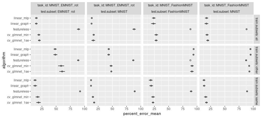
The plot above shows means and standard deviations for all the models.
Does training on the other subset work?
We focus only on predicting MNIST, after training on another data set.
score_other <- score_stats[test.subset=="MNIST" & train.subsets=="other"]
ggplot()+
  geom_point(aes(
    percent_error_mean, algorithm),
    shape=1,
    data=score_other)+
  geom_segment(aes(
    percent_error_mean+percent_error_sd, algorithm,
    xend=percent_error_mean-percent_error_sd, yend=algorithm),
    data=score_other)+
  facet_grid(. ~ task_id, labeller=label_both)+
  scale_x_continuous(
    "Test error on MNIST (mean +/- SD over 3 folds), after training on Other subset (EMNIST/Fashion)",
    limits=c(40,100),
    breaks=seq(40,100,by=10))
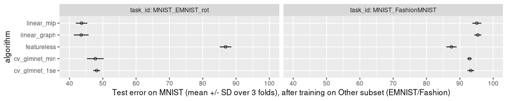
The figure above shows that
- training on
EMNIST_rothas significantly smaller error rates than featureless, indicating that these data are similar enough to MNIST, for the linear model to be able to learn something useful. - torch linear models are a bit more accurate than
cv_glmnet(surprising, since both are linear models). - there is not much difference between the two torch linear models (as expected).
- there is not much difference between the two
cv_glmnetlinear models (as expected), although the min variant has a slightly smaller error rate (as expected). - training on
FashionMNISThas significantly larger error rates than featureless, indicating that the data are so different, that the linear model does not learn anything relevant for accurate predictions on the other subset.
Comparing Other and Same
Is training on EMNIST as good as training on MNIST, if our goal is good predictions in MNIST?
score_EMNIST <- score_stats[test.subset=="MNIST" & task_id=="MNIST_EMNIST_rot"]
ggplot()+
  ggtitle("SOAK results for MNIST_EMNIST_rot data")+
  geom_point(aes(
    percent_error_mean, algorithm,
    color=train.subsets),
    shape=1,
    data=score_EMNIST)+
  geom_segment(aes(
    percent_error_mean+percent_error_sd, algorithm,
    color=train.subsets,
    xend=percent_error_mean-percent_error_sd, yend=algorithm),
    data=score_EMNIST)+
  scale_x_continuous(
    "Test error on MNIST (mean +/- SD over 3 folds)",
    limits=c(0,100),
    breaks=seq(0,100,by=10))
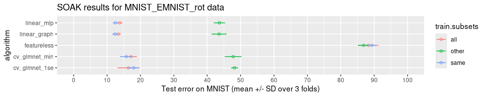
The figure above indicates that the Other model (training on EMNIST) has much larger error rates, compared to the Same model (training on MNIST). These data indicate that the data subsets are not similar enough for the linear model to fully generalize between subsets.
Early stopping diagnostic plot
For each of the models we can check if the early stopping regularization worked reasonably, via code as below.
one.glearner <- score_dt[algorithm=="linear_graph"]$learner[[1]]
glearner_model <- one.glearner$archive$learners(1)[[1]]$model
(glearner_long <- melt_history(
  glearner_model$torch_model_classif$model$callbacks$history))
##       epoch        set    measure     value
##       <num>     <fctr>     <fctr>     <num>
##    1:     1   subtrain    logloss 2.1998343
##    2:     2   subtrain    logloss 1.8533952
##    3:     3   subtrain    logloss 1.6084012
##    4:     4   subtrain    logloss 1.4168391
##    5:     5   subtrain    logloss 1.2765990
##   ---
## 3996:   996 validation error_prop 0.1879699
## 3997:   997 validation error_prop 0.1879699
## 3998:   998 validation error_prop 0.1879699
## 3999:   999 validation error_prop 0.1879699
## 4000:  1000 validation error_prop 0.1894737
(glearner_selected <- as.data.table(
  one.glearner$tuning_result$internal_tuned_values[[1]]))
##    torch_model_classif.epochs
##                         <int>
## 1:                        195
ggplot()+
  facet_grid(measure ~ ., scales="free")+
  geom_vline(aes(
    xintercept=torch_model_classif.epochs),
    data=glearner_selected)+
  geom_line(aes(
    epoch, value, color=set),
    data=glearner_long)
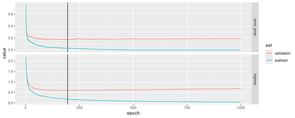
The figure above shows typical subtrain/validation error curves, with an optimal number of epochs chosen reasonably (an intermediate value that minimizes the log loss).
Conclusions
We have shown two ways that mlr3torch can be used to define a linear model (either using MLP learner or via pipe operations), and we showed how it can simplify learning code, relative to using torch by itself (requires coding a for loop over epochs). We also showed how to run machine learning benchmark experiments in parallel, then interpret results using figures.
Session info
sessionInfo()
## R version 4.4.3 (2025-02-28)
## Platform: x86_64-pc-linux-gnu
## Running under: Ubuntu 24.04.2 LTS
##
## Matrix products: default
## BLAS:   /usr/lib/x86_64-linux-gnu/blas/libblas.so.3.12.0
## LAPACK: /usr/lib/x86_64-linux-gnu/lapack/liblapack.so.3.12.0
##
## locale:
##  [1] LC_CTYPE=fr_FR.UTF-8       LC_NUMERIC=C               LC_TIME=fr_FR.UTF-8        LC_COLLATE=fr_FR.UTF-8
##  [5] LC_MONETARY=fr_FR.UTF-8    LC_MESSAGES=fr_FR.UTF-8    LC_PAPER=fr_FR.UTF-8       LC_NAME=C
##  [9] LC_ADDRESS=C               LC_TELEPHONE=C             LC_MEASUREMENT=fr_FR.UTF-8 LC_IDENTIFICATION=C
##
## time zone: Europe/Paris
## tzcode source: system (glibc)
##
## attached base packages:
## [1] stats     graphics  grDevices utils     datasets  methods   base
##
## other attached packages:
## [1] mlr3resampling_2024.10.28 mlr3_0.23.0               ggplot2_3.5.1             data.table_1.17.99
##
## loaded via a namespace (and not attached):
##  [1] future_1.34.0        shape_1.4.6.1        lattice_0.22-6       listenv_0.9.1        digest_0.6.37
##  [6] magrittr_2.0.3       evaluate_1.0.3       grid_4.4.3           iterators_1.0.14     foreach_1.5.2
## [11] glmnet_4.1-8         Matrix_1.7-3         processx_3.8.6       backports_1.5.0      mlr3learners_0.10.0
## [16] survival_3.8-3       torch_0.14.2         ps_1.9.0             scales_1.3.0         coro_1.1.0
## [21] mlr3tuning_1.3.0     mlr3measures_1.0.0   codetools_0.2-20     palmerpenguins_0.1.1 cli_3.6.4
## [26] crayon_1.5.3         rlang_1.1.5          future.apply_1.11.3  parallelly_1.42.0    bit64_4.6.0-1
## [31] munsell_0.5.1        splines_4.4.3        withr_3.0.2          nc_2025.1.21         mlr3pipelines_0.7.2
## [36] tools_4.4.3          parallel_4.4.3       uuid_1.2-1           checkmate_2.3.2      colorspace_2.1-1
## [41] globals_0.16.3       bbotk_1.5.0          vctrs_0.6.5          R6_2.6.1             lifecycle_1.0.4
## [46] bit_4.6.0            mlr3misc_0.16.0      pkgconfig_2.0.3      callr_3.7.6          pillar_1.10.1
## [51] gtable_0.3.6         glue_1.8.0           Rcpp_1.0.14          lgr_0.4.4            paradox_1.0.1
## [56] xfun_0.51            tibble_3.2.1         knitr_1.50           farver_2.1.2         labeling_0.4.3
## [61] compiler_4.4.3       mlr3torch_0.2.1