Generalization to new subsets in R
The goal of this blog post is to explain how to quantify the extent to which it is possible to train on one data subset (say a geographic region such as Europe), and predict on another data subset (say North America). The ideas are similar to my previous python blog, but the code below is in R.
Simulated data
Assume there is a data set with 1000 rows,
N <- 1000
library(data.table)
## data.table 1.14.99 IN DEVELOPMENT built 2023-12-18 16:20:35 UTC using 6 threads (see ?getDTthreads). Latest news: r-datatable.com
(full.dt <- data.table(
  label=factor(rep(c("burned","no burn"), l=N)),
  image=c(rep(1, 0.4*N), rep(2, 0.4*N), rep(3, 0.1*N), rep(4, 0.1*N))
)[, signal := ifelse(label=="no burn", 0, 1)*image][])
##         label image signal
##        <fctr> <num>  <num>
##    1:  burned     1      1
##    2: no burn     1      0
##    3:  burned     1      1
##    4: no burn     1      0
##    5:  burned     1      1
##   ---
##  996: no burn     4      0
##  997:  burned     4      4
##  998: no burn     4      0
##  999:  burned     4      4
## 1000: no burn     4      0
Above each row has an image ID between 1 and 4. We also generate/simulate some features:
set.seed(1)
n.images <- length(unique(full.dt$image))
for(image.i in 1:n.images){
  set(full.dt, j=paste0("feature_easy_noise",image.i), value=rnorm(N))
  full.dt[, paste0("feature_impossible",image.i) := ifelse(
    image==image.i, signal, 0)+rnorm(N)]
}
set(full.dt, j="feature_easy_signal", value=rnorm(N)+full.dt$signal)
str(full.dt)
## Classes 'data.table' and 'data.frame':	1000 obs. of  12 variables:
##  $ label              : Factor w/ 2 levels "burned","no burn": 1 2 1 2 1 2 1 2 1 2 ...
##  $ image              : num  1 1 1 1 1 1 1 1 1 1 ...
##  $ signal             : num  1 0 1 0 1 0 1 0 1 0 ...
##  $ feature_easy_noise1: num  -0.626 0.184 -0.836 1.595 0.33 ...
##  $ feature_impossible1: num  2.135 1.112 0.129 0.211 1.069 ...
##  $ feature_easy_noise2: num  -0.8861 -1.9223 1.6197 0.5193 -0.0558 ...
##  $ feature_impossible2: num  0.739 0.387 1.296 -0.804 -1.603 ...
##  $ feature_easy_noise3: num  -1.135 0.765 0.571 -1.352 -2.03 ...
##  $ feature_impossible3: num  -1.516 0.629 -1.678 1.18 1.118 ...
##  $ feature_easy_noise4: num  -0.6188 -1.1094 -2.1703 -0.0313 -0.2604 ...
##  $ feature_impossible4: num  -1.325 0.952 0.86 1.061 -0.351 ...
##  $ feature_easy_signal: num  1.264 -0.829 -0.462 1.684 -0.544 ...
##  - attr(*, ".internal.selfref")=<externalptr>
There are two sets of four features:
- For easy features, four are random noise (
feature_easy_noise1etc), and one is correlated with the label (feature_easy_signal), so the algorithm just needs to learn to ignore the noise features, and concentrate on the signal feature. That should be possible given data from any image (same signal in each image). - Each impossible feature is correlated with the label (when feature
number same as image number), or is just noise (when image number
different from feature number). So if the algorithm has access to
the correct image (same as test, say image 2), then it needs to
learn to use the corresponding feature
feature_impossible2. But if the algorithm does not have access to that image, then the best it can do is same as featureless (predict most frequent class label in train data).
The signal is stronger for larger image numbers (image number 4 is easier to learn from than image number 1).
Assign cross-validation folds
We would like to fix a test image, and then compare models trained on either the same image, or on different images (or all images). To create a K-fold cross-validation experiment (say K=3 folds), we therefore need to assign fold IDs in a way such that each image is present in each fold. One way to do that would be to just use random integers,
n.folds <- 3
set.seed(1)
full.dt[
, random.fold := sample(n.folds, size=N, replace=TRUE)
][, table(random.fold, image)]
##            image
## random.fold   1   2   3   4
##           1 147 144  27  33
##           2 125 143  37  34
##           3 128 113  36  33
In the output above we see that for each image, there is not an equal number of data assigned to each fold. How could we do that?
uniq.folds <- 1:n.folds
full.dt[
, fold := sample(rep(uniq.folds, l=.N)), by=image
][, table(fold, image)]
##     image
## fold   1   2   3   4
##    1 134 134  34  34
##    2 133 133  33  33
##    3 133 133  33  33
The table above shows that for each image, the number of data per fold is equal (or off by one). The first method of fold assignment above is called simple random sampling, and the second is called stratified random sampling, which can also be implemented in mlr3.
We can visualize the different split sets using these fold IDs with a for loop:
for(test.fold in uniq.folds){
  full.dt[, set := ifelse(fold==test.fold, "test", "train")]
  cat("\nSplit=",test.fold,"\n")
  print(dcast(full.dt, fold + set ~ image, length))
}
##
## Split= 1
## Key: <fold, set>
##     fold    set     1     2     3     4
##    <int> <char> <int> <int> <int> <int>
## 1:     1   test   134   134    34    34
## 2:     2  train   133   133    33    33
## 3:     3  train   133   133    33    33
##
## Split= 2
## Key: <fold, set>
##     fold    set     1     2     3     4
##    <int> <char> <int> <int> <int> <int>
## 1:     1  train   134   134    34    34
## 2:     2   test   133   133    33    33
## 3:     3  train   133   133    33    33
##
## Split= 3
## Key: <fold, set>
##     fold    set     1     2     3     4
##    <int> <char> <int> <int> <int> <int>
## 1:     1  train   134   134    34    34
## 2:     2  train   133   133    33    33
## 3:     3   test   133   133    33    33
The output above indicates that there are equal proportions of each image in each set (train and test). So we can fix a test fold, say 2, and also a test image, say 4. Then there are 33 data points in that test set. We can try to predict them by using machine learning algorithms on several different train sets:
- same: train folds (3 and 1) and same image (4), there are 34+33=67 train data in this set.
- other: train folds (3 and 1) and other images (1-3), there are 601 train data in this set.
- all: train folds (3 and 1) and all images (1-4), there are 668 train data in this set.
For each of the three trained models, we compute prediction error on the test set (image 4, fold 2), then compare the error rates to determine how much error changes when we train on a different set of images.
- Because there are relatively few data from image 4, it may be beneficial to train on a larger data set (including images 1-3), even if those data are somewhat different. (and other/all error may actually be smaller than same error)
- Conversely, if the data in images 1-3 are substantially different, then it may not help at all to use different images. (in this case, same error would be smaller than other/all error)
Typically if there are a reasonable number of train data, the same model should do better than other/all, but you have to do the computational experiment to find out what is true for your particular data set.
Define train and test sets
The code below defines a table with one row for each train/test split.
feature.types <- c("easy","impossible")
(split.dt <- data.table::CJ(
  test.fold=uniq.folds,
  test.image=1:n.images,
  train.name=c("same","other","all"),
  features=feature.types))
## Key: <test.fold, test.image, train.name, features>
##     test.fold test.image train.name   features
##         <int>      <int>     <char>     <char>
##  1:         1          1        all       easy
##  2:         1          1        all impossible
##  3:         1          1      other       easy
##  4:         1          1      other impossible
##  5:         1          1       same       easy
##  6:         1          1       same impossible
##  7:         1          2        all       easy
##  8:         1          2        all impossible
##  9:         1          2      other       easy
## 10:         1          2      other impossible
## 11:         1          2       same       easy
## 12:         1          2       same impossible
## 13:         1          3        all       easy
## 14:         1          3        all impossible
## 15:         1          3      other       easy
## 16:         1          3      other impossible
## 17:         1          3       same       easy
## 18:         1          3       same impossible
## 19:         1          4        all       easy
## 20:         1          4        all impossible
## 21:         1          4      other       easy
## 22:         1          4      other impossible
## 23:         1          4       same       easy
## 24:         1          4       same impossible
## 25:         2          1        all       easy
## 26:         2          1        all impossible
## 27:         2          1      other       easy
## 28:         2          1      other impossible
## 29:         2          1       same       easy
## 30:         2          1       same impossible
## 31:         2          2        all       easy
## 32:         2          2        all impossible
## 33:         2          2      other       easy
## 34:         2          2      other impossible
## 35:         2          2       same       easy
## 36:         2          2       same impossible
## 37:         2          3        all       easy
## 38:         2          3        all impossible
## 39:         2          3      other       easy
## 40:         2          3      other impossible
## 41:         2          3       same       easy
## 42:         2          3       same impossible
## 43:         2          4        all       easy
## 44:         2          4        all impossible
## 45:         2          4      other       easy
## 46:         2          4      other impossible
## 47:         2          4       same       easy
## 48:         2          4       same impossible
## 49:         3          1        all       easy
## 50:         3          1        all impossible
## 51:         3          1      other       easy
## 52:         3          1      other impossible
## 53:         3          1       same       easy
## 54:         3          1       same impossible
## 55:         3          2        all       easy
## 56:         3          2        all impossible
## 57:         3          2      other       easy
## 58:         3          2      other impossible
## 59:         3          2       same       easy
## 60:         3          2       same impossible
## 61:         3          3        all       easy
## 62:         3          3        all impossible
## 63:         3          3      other       easy
## 64:         3          3      other impossible
## 65:         3          3       same       easy
## 66:         3          3       same impossible
## 67:         3          4        all       easy
## 68:         3          4        all impossible
## 69:         3          4      other       easy
## 70:         3          4      other impossible
## 71:         3          4       same       easy
## 72:         3          4       same impossible
##     test.fold test.image train.name   features
The table above has a row for every unique combination of test fold, test image, train set name, and data set input features. Why do we need a separate column for test fold and test image? We are interested to see the extent to which it is possible to train on one image (say, from Europe), and test on another image (say, from North America). We therefore fix one image as the test image, and we would like to compare how two different models predict on this image: (1) one model trained on the same image, (2) another model trained on other images. We therefore need to assign data from each image into folds, so that we can train on data from the same image, while setting some of the data from this image aside as a test set.
The code below computes data tables with indices of train and test sets for all of the splits in the experiment.
get_set_list <- function(data.dt, split.info){
  out.list <- list()
  is.set.image <- list(
    test=data.dt[["image"]] == split.info[["test.image"]])
  is.set.image[["train"]] <- switch(
    split.info[["train.name"]],
    same=is.set.image[["test"]],
    other=!is.set.image[["test"]],
    all=rep(TRUE, nrow(data.dt)))
  is.set.fold <- list(
    test=data.dt[["fold"]] == split.info[["test.fold"]])
  is.set.fold[["train"]] <- !is.set.fold[["test"]]
  for(set in names(is.set.fold)){
    is.image <- is.set.image[[set]]
    is.fold <- is.set.fold[[set]]
    out.list[[set]] <- data.dt[is.image & is.fold]
  }
  out.list
}
easy.dt <- setkey(split.dt[features=="easy"], train.name, test.image, test.fold)
(one.easy <- easy.dt[1])
## Key: <train.name, test.image, test.fold>
##    test.fold test.image train.name features
##        <int>      <int>     <char>   <char>
## 1:         1          1        all     easy
meta.dt <- setkey(full.dt[, .(image, fold)])[, row := .I]
(train.test.list <- get_set_list(meta.dt, one.easy))
## $test
## Key: <image, fold>
##      image  fold   row
##      <num> <int> <int>
##   1:     1     1     1
##   2:     1     1     2
##   3:     1     1     3
##   4:     1     1     4
##   5:     1     1     5
##  ---
## 130:     1     1   130
## 131:     1     1   131
## 132:     1     1   132
## 133:     1     1   133
## 134:     1     1   134
##
## $train
## Key: <image, fold>
##      image  fold   row
##      <num> <int> <int>
##   1:     1     2   135
##   2:     1     2   136
##   3:     1     2   137
##   4:     1     2   138
##   5:     1     2   139
##  ---
## 660:     4     3   996
## 661:     4     3   997
## 662:     4     3   998
## 663:     4     3   999
## 664:     4     3  1000
The function get_set_list returns a list with named elements train
and test, each of which is a data table with one row per data point
to use for either training or testing in a particular split. Below, we
summarize those tables, by condensing contiguous runs of rows into a
single row with start/end columns.
point2seg <- function(DT){
  mid.end.i <- data.table(DT)[
  , diff := c(diff(row),NA)
  ][,which(diff!=1)]
  start.i <- c(1,mid.end.i+1)
  DT[, .(
    DT[start.i],
    start=row[start.i],
    end=row[c(mid.end.i,.N)]
  )]
}
lapply(train.test.list, point2seg)
## $test
## Key: <image, fold>
##    image  fold   row start   end
##    <num> <int> <int> <int> <int>
## 1:     1     1     1     1   134
##
## $train
## Key: <image, fold>
##    image  fold   row start   end
##    <num> <int> <int> <int> <int>
## 1:     1     2   135   135   400
## 2:     2     2   535   535   800
## 3:     3     2   835   835   900
## 4:     4     2   935   935  1000
The result above shows that there are four contiguous runs of data to train on (from row 135 to 400, 535 to 800, etc), whereas there is a single contiguous run of test data (from row 1 to 134). In the code below, we use these two functions to construct a single table that describes all of the train and test splits in our computational cross-validation experiment.
index.dt.list <- list()
for(split.i in 1:nrow(easy.dt)){
  split.row <- easy.dt[split.i]
  meta.set.list <- get_set_list(meta.dt, split.row)
  for(set in names(meta.set.list)){
    point.dt <- meta.set.list[[set]]
    seg.dt <- point2seg(point.dt)
    index.dt.list[[paste(split.i, set)]] <- data.table(
      split.i, set, split.row, seg.dt)
  }
}
(index.dt <- data.table::rbindlist(index.dt.list))
##      split.i    set test.fold test.image train.name features image  fold   row start   end
##        <int> <char>     <int>      <int>     <char>   <char> <num> <int> <int> <int> <int>
##   1:       1   test         1          1        all     easy     1     1     1     1   134
##   2:       1  train         1          1        all     easy     1     2   135   135   400
##   3:       1  train         1          1        all     easy     2     2   535   535   800
##   4:       1  train         1          1        all     easy     3     2   835   835   900
##   5:       1  train         1          1        all     easy     4     2   935   935  1000
##  ---
## 142:      35   test         2          4       same     easy     4     2   935   935   967
## 143:      35  train         2          4       same     easy     4     1   901   901   934
## 144:      35  train         2          4       same     easy     4     3   968   968  1000
## 145:      36   test         3          4       same     easy     4     3   968   968  1000
## 146:      36  train         3          4       same     easy     4     1   901   901   967
There is one row in the table above for every contiguous block of data in each set (assuming rows are sorted by image and then fold). These data are visualized below,
library(ggplot2)
rect.expand <- 0.25
image.rows <- rbind(
  meta.dt[, .(group="image", min.row=min(row), max.row=max(row)), by=image][, fold := NA],
  meta.dt[, .(group="fold", min.row=min(row), max.row=max(row)), by=.(image, fold)])
ggplot()+
  ggtitle("All train/test splits to compute")+
  theme_bw()+
  facet_grid(. ~ train.name, labeller=label_both, scales="free", space="free")+
  scale_size_manual(values=c(image=3, fold=1))+
  scale_color_manual(values=c(image="black", fold="grey50"))+
  geom_rect(aes(
    xmin=-Inf, xmax=Inf,
    color=group,
    size=group,
    ymin=min.row, ymax=max.row),
    fill=NA,
    data=image.rows)+
  geom_rect(aes(
    xmin=split.i-rect.expand, ymin=start,
    xmax=split.i+rect.expand, ymax=end,
    fill=set),
    data=index.dt)+
  geom_text(aes(
    ifelse(group=="image", 25, 36),
    (min.row+max.row)/2,
    hjust=ifelse(group=="image", 0, 1),
    label=sprintf("%s=%d", group, ifelse(group=="image", image, fold))),
    data=data.table(train.name="same", image.rows))+
  scale_x_continuous(
    "Split number", breaks=seq(0, 100, by=2))+
  scale_y_continuous(
    "Row number (data sorted by image, fold)")
## Warning: Using `size` aesthetic for lines was deprecated in ggplot2 3.4.0.
## ℹ Please use `linewidth` instead.
## This warning is displayed once every 8 hours.
## Call `lifecycle::last_lifecycle_warnings()` to see where this warning was generated.
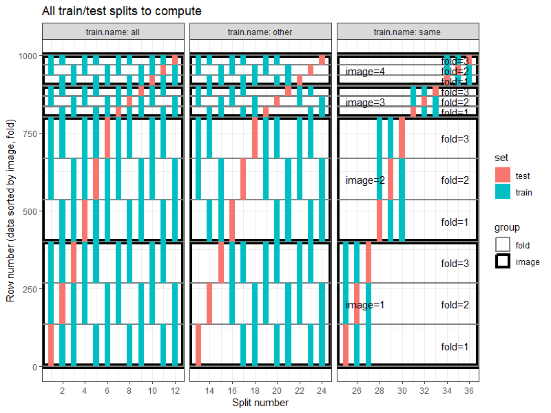
The plot above shows all splits to compute. Each panel shows the splits for one kind of train set (all, other, or same).
- The
allpanel shows what happens when testing on a given image, and training on all images (including the same image). Example: Split number 12 is testing on image 4, test fold 3, training on test folds 1-2 from all four images. - The
otherpanel shows what happens when testing on a given image, but training on other images (not the same image). Example: Split number 24 is testing on image 4, test fold 3, training on test folds 1-2 from other three images. - The
samepanel shows the usual cross-validation setup run on each image separately. Train on one image, test on same image (but not the same rows/data). Example: Split number 36 is testing on image 4, test fold 3, training on test folds 1-2 from same image (number 4).
The plot below emphasizes the differences between the three train sets, for a particular test image, and for each fold. Note that the split numbers in the plot below are not the same as in the plot above.
target.image <- 2
some.split.test <- setkey(index.dt[set=="test" & image==target.image], fold, train.name)[
, new.split.i := .I]
some.indices <- index.dt[some.split.test[, .(new.split.i, split.i)], on="split.i"]
ggplot()+
  ggtitle(paste0("Train/test splits to compute for image=", target.image))+
  theme_bw()+
  scale_size_manual(values=c(image=3, fold=1))+
  scale_color_manual(values=c(image="black", fold="grey50"))+
  facet_grid(. ~ test.fold, labeller=label_both, scales="free", space="free")+
  geom_rect(aes(
    xmin=-Inf, xmax=Inf,
    color=group,
    size=group,
    ymin=min.row, ymax=max.row),
    fill=NA,
    data=image.rows)+
  geom_rect(aes(
    xmin=new.split.i-rect.expand, ymin=start,
    xmax=new.split.i+rect.expand, ymax=end,
    fill=set),
    data=some.indices)+
  geom_text(aes(
    ifelse(group=="image", 1.5, 2.5),
    (min.row+max.row)/2,
    label=sprintf("%s=%d", group, ifelse(group=="image", image, fold))),
    data=data.table(test.fold=1, image.rows))+
  geom_text(aes(
    new.split.i, Inf, label=train.name),
    vjust=1.2,
    data=some.split.test)+
  scale_x_continuous(
    "Split number", breaks=seq(0, 100, by=1))+
  scale_y_continuous(
    "Row number (data sorted by image, fold)")
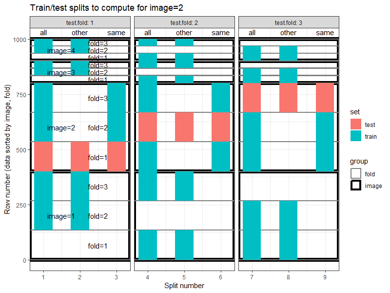
The plot above shows three panels, one for each test fold. In each panel the difference between the three train sets (all, other, same) is clear.
For loop
The code to compute test accuracy for one of the splits should look something like below,
OneSplit <- function(test.fold, test.image, train.name, features){
  split.meta <- data.table(test.fold, test.image, train.name, features)
  full.set.list <- get_set_list(full.dt, split.meta)
  X.list <- list()
  y.list <- list()
  for(set in names(full.set.list)){
    set.dt <- full.set.list[[set]]
    feature.name.vec <- grep(
      features, names(set.dt), value=TRUE, fixed=TRUE)
    X.list[[set]] <- as.matrix(set.dt[, feature.name.vec, with=FALSE])
    y.list[[set]] <- set.dt[["label"]]
  }
  fit <- glmnet::cv.glmnet(X.list[["train"]], y.list[["train"]], family="binomial")
  most.freq.label <- full.set.list[["train"]][
  , .(count=.N), by=label
  ][order(-count), paste(label)][1]
  set.seed(1)
  pred.list <- list(
    cv.glmnet=paste(predict(fit, X.list[["test"]], type="class")),
    featureless=rep(most.freq.label, nrow(X.list[["test"]])))
  acc.dt.list <- list()
  for(pred.name in names(pred.list)){
    pred.vec <- pred.list[[pred.name]]
    is.correct <- pred.vec==y.list[["test"]]
    acc.dt.list[[paste(pred.name)]] <- data.table(
      pred.name,
      accuracy.percent=100*mean(is.correct))
  }
  data.table(split.meta, rbindlist(acc.dt.list))
}
do.call(OneSplit, split.dt[1])
##    test.fold test.image train.name features   pred.name accuracy.percent
##        <int>      <int>     <char>   <char>      <char>            <num>
## 1:         1          1        all     easy   cv.glmnet         65.67164
## 2:         1          1        all     easy featureless         47.76119
The code above uses a helper function OneSplit which is to be called
with meta data from one of the rows of split.dt. Below I do the computation in sequence on my
personal computer,
loop.acc.dt.list <- list()
for(split.i in 1:nrow(split.dt)){
  split.row <- split.dt[split.i]
  loop.acc.dt.list[[split.i]] <- do.call(OneSplit, split.row)
}
(loop.acc.dt <- rbindlist(loop.acc.dt.list))
##      test.fold test.image train.name   features   pred.name accuracy.percent
##          <int>      <int>     <char>     <char>      <char>            <num>
##   1:         1          1        all       easy   cv.glmnet         65.67164
##   2:         1          1        all       easy featureless         47.76119
##   3:         1          1        all impossible   cv.glmnet         57.46269
##   4:         1          1        all impossible featureless         47.76119
##   5:         1          1      other       easy   cv.glmnet         61.94030
##  ---
## 140:         3          4      other impossible featureless         60.60606
## 141:         3          4       same       easy   cv.glmnet         96.96970
## 142:         3          4       same       easy featureless         39.39394
## 143:         3          4       same impossible   cv.glmnet         96.96970
## 144:         3          4       same impossible featureless         39.39394
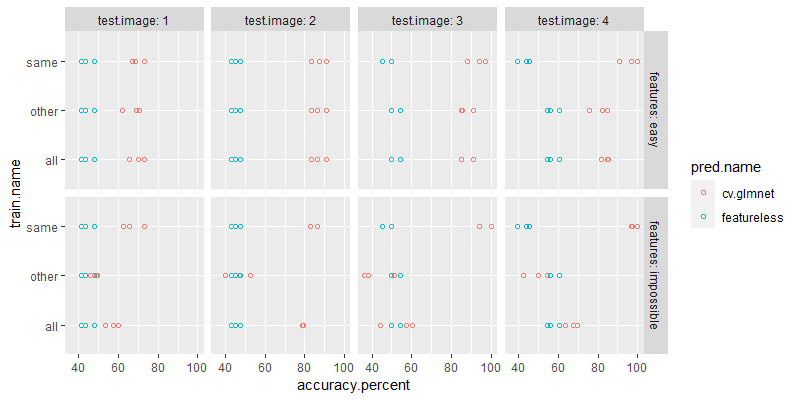
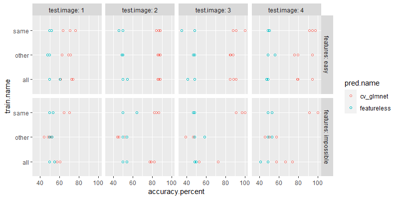
Below we plot the accuracy numbers,
ggplot()+
  geom_point(aes(
    accuracy.percent, train.name, color=pred.name),
    shape=1,
    data=loop.acc.dt)+
  facet_grid(features ~ test.image, labeller=label_both)
Parallelization
The result for each split can be computed in parallel. Below I do the computation in parallel on my personal computer, by declaring a future plan, and then using future_lapply:
future::plan("multisession")
future.acc.dt.list <- future.apply::future_lapply(1:nrow(split.dt), function(split.i){
  split.row <- split.dt[split.i]
  do.call(OneSplit, split.row)
}, future.seed=TRUE)
(future.acc.dt <- rbindlist(future.acc.dt.list))
##      test.fold test.image train.name   features   pred.name accuracy.percent
##          <int>      <int>     <char>     <char>      <char>            <num>
##   1:         1          1        all       easy   cv.glmnet         65.67164
##   2:         1          1        all       easy featureless         47.76119
##   3:         1          1        all impossible   cv.glmnet         57.46269
##   4:         1          1        all impossible featureless         47.76119
##   5:         1          1      other       easy   cv.glmnet         61.94030
##  ---
## 140:         3          4      other impossible featureless         60.60606
## 141:         3          4       same       easy   cv.glmnet         96.96970
## 142:         3          4       same       easy featureless         39.39394
## 143:         3          4       same impossible   cv.glmnet         96.96970
## 144:         3          4       same impossible featureless         39.39394
Below we plot the accuracy numbers,
ggplot()+
  geom_point(aes(
    accuracy.percent, train.name, color=pred.name),
    shape=1,
    data=future.acc.dt)+
  facet_grid(features ~ test.image, labeller=label_both)
Exercise for the reader: do the same computation on a cluster such as NAU Monsoon, using batchtools or future.batchtools.
mlr3 with ResamplingCustom
In this section we show how it is possible using mlr3::ResamplingCustom to do the same computations as we did above. First we turn off logging, to reduce noisy output:
lgr::get_logger("mlr3")$set_threshold("warn")
Then we use for loops over splits with mlr3 custom resampling:
bench.acc.dt.list <- list()
for(feat in feature.types){
  feature.name.vec <- grep(
    feat, names(full.dt), value=TRUE, fixed=TRUE)
  some.dt <- full.dt[, c("label", feature.name.vec), with=FALSE]
  task <- mlr3::TaskClassif$new(feat, some.dt, target="label")
  split.feat <- split.dt[features==feat]
  for(split.i in 1:nrow(split.feat)){
    split.row <- split.feat[split.i]
    full.set.list <- get_set_list(meta.dt, split.row)
    split.feat[
      split.i,
      names(full.set.list) := lapply(
        full.set.list, function(DT)list(DT$row)
      )
    ]
  }
  score.dt <- split.feat[, {
    custom <- mlr3::rsmp("custom")
    custom$instantiate(task, train, test)
    benchmark.design <- mlr3::benchmark_grid(
      task,
      list(
        mlr3learners::LearnerClassifCVGlmnet$new(),
        mlr3::LearnerClassifFeatureless$new()),
      custom)
    benchmark.result <- mlr3::benchmark(benchmark.design)
    benchmark.result$score()
  }, by=.(test.image, train.name)]
  bench.acc.dt.list[[feat]] <- score.dt[, .(
    test.fold=iteration,
    test.image,
    train.name,
    features=feat,
    pred.name=sub("classif.", "", learner_id, fixed=TRUE),
    accuracy.percent=100*(1-classif.ce))]
}
(bench.acc.dt <- data.table::rbindlist(bench.acc.dt.list))
##      test.fold test.image train.name   features   pred.name accuracy.percent
##          <int>      <int>     <char>     <char>      <char>            <num>
##   1:         1          1        all       easy   cv_glmnet         73.88060
##   2:         2          1        all       easy   cv_glmnet         60.90226
##   3:         3          1        all       easy   cv_glmnet         72.18045
##   4:         1          1        all       easy featureless         60.44776
##   5:         2          1        all       easy featureless         49.62406
##  ---
## 140:         2          4       same impossible   cv_glmnet        100.00000
## 141:         3          4       same impossible   cv_glmnet         90.90909
## 142:         1          4       same impossible featureless         52.94118
## 143:         2          4       same impossible featureless         48.48485
## 144:         3          4       same impossible featureless         48.48485
The mlr3 code above is more or less the same size/complexity as the
OneSplit function we defined previously in the section using for
loops. Implementing this kind of cross-validation is not significantly
easier, using mlr3, compared to base R. The results are visualized below:
ggplot()+
  geom_point(aes(
    accuracy.percent, train.name, color=pred.name),
    shape=1,
    data=bench.acc.dt)+
  facet_grid(features ~ test.image, labeller=label_both)
Exercise for the reader: parallelize the mlr3 computation by using
future::plan("multisession").
Is it possible to implement this using existing mlr3 classes? No.
Using mlr3 would be easier if there was a different kind of Resampling class that supported the kind of cross-validation experiment we have implemented above.
strat.dt <- full.dt[, c("label", "image", feature.name.vec), with=FALSE]
tsk_str = mlr3::TaskClassif$new(feat, strat.dt, target="label")
tsk_str$set_col_roles("label", c("target", "stratum"))
tsk_str$set_col_roles("image", "stratum")
tsk_grp = mlr3::TaskClassif$new(feat, strat.dt, target="label")
tsk_grp$set_col_roles("image", "group")
task.list <- list(stratified=tsk_str, random=task, grouped=tsk_grp)
rsmp_cv3 = mlr3::rsmp("cv", folds = n.folds)

sampling.dt.list <- list()
set.seed(1)
for(sampling.type in names(task.list)){
  sampling.task <- task.list[[sampling.type]]
  rsmp_cv3$instantiate(sampling.task)
  for(test.fold in uniq.folds){
    test.i <- rsmp_cv3$test_set(test.fold)
    sampling.dt.list[[paste(
      sampling.type, test.fold
    )]] <- data.table(
      sampling.type, test.fold,
      strat.dt[test.i]
    )
  }
}
sampling.dt <- data.table::rbindlist(sampling.dt.list)
data.table::dcast(
  sampling.dt,
  sampling.type + label + test.fold ~ image,
  length)
## Key: <sampling.type, label, test.fold>
##     sampling.type   label test.fold     1     2     3     4
##            <char>  <fctr>     <int> <int> <int> <int> <int>
##  1:       grouped  burned         1     0     0    50    50
##  2:       grouped  burned         2   200     0     0     0
##  3:       grouped  burned         3     0   200     0     0
##  4:       grouped no burn         1     0     0    50    50
##  5:       grouped no burn         2   200     0     0     0
##  6:       grouped no burn         3     0   200     0     0
##  7:        random  burned         1    75    61    16    10
##  8:        random  burned         2    56    68    15    21
##  9:        random  burned         3    69    71    19    19
## 10:        random no burn         1    66    69    20    17
## 11:        random no burn         2    81    65    10    17
## 12:        random no burn         3    53    66    20    16
## 13:    stratified  burned         1    67    67    17    17
## 14:    stratified  burned         2    67    67    17    17
## 15:    stratified  burned         3    66    66    16    16
## 16:    stratified no burn         1    67    67    17    17
## 17:    stratified no burn         2    67    67    17    17
## 18:    stratified no burn         3    66    66    16    16
The table above shows the number of data points/labels assigned to each test fold, for each image and sampling type.
- In the first 6 rows of the table above (grouped sampling), we see that data from each image have all been assigned to a single test fold.
- In the second 6 rows (random sampling), we see that there are not necessarily equal numbers of samples of each class/image, across folds.
- In the bottom 6 rows (stratified sampling), we see that there are equal numbers of samples of each class/image (up to a difference of 1), across folds.
Where is this stratification implemented? Inside instantiate method
of
Resampling,
it uses strata element:
tsk_str$strata
##        N                      row_id
##    <int>                      <list>
## 1:   200        1, 3, 5, 7, 9,11,...
## 2:   200        2, 4, 6, 8,10,12,...
## 3:   200 401,403,405,407,409,411,...
## 4:   200 402,404,406,408,410,412,...
## 5:    50 801,803,805,807,809,811,...
## 6:    50 802,804,806,808,810,812,...
## 7:    50 901,903,905,907,909,911,...
## 8:    50 902,904,906,908,910,912,...
Grouped
Resampling
is a mlr3 concept which is related to the idea we explored in this
blog post. It is implemented via tsk_grp$set_col_roles("year",
"group") which makes sure that resampling will not put any items from
the same group in different sets. So we could use that for quantifying
the accuracy of training on one image, and testing on another
image. There is an error message in the source
code
stopf("Cannot combine stratification with grouping"), why not? On
that page in the doc comments it is also written that instance is an
internal object that may not necessarily be the row ids of the
original data:
 #' @field instance (any)\cr
    #'   During `instantiate()`, the instance is stored in this slot in an arbitrary format.
    #'   Note that if a grouping variable is present in the [Task], a [Resampling] may operate on the
    #'   group ids internally instead of the row ids (which may lead to confusion).
    #'
    #'   It is advised to not work directly with the `instance`, but instead only use the getters
    #'   `$train_set()` and `$test_set()`.
Below we show the instance element for each task,
lapply(task.list, function(my_task){
  rsmp_cv3$instantiate(my_task)
  rsmp_cv3$instance
})
## $stratified
##       row_id  fold
##        <int> <int>
##    1:      1     1
##    2:      5     1
##    3:      7     1
##    4:      9     1
##    5:     15     1
##   ---
##  996:    984     3
##  997:    986     3
##  998:    994     3
##  999:    996     3
## 1000:    998     3
##
## $random
## Key: <fold>
##       row_id  fold
##        <int> <int>
##    1:      2     1
##    2:      4     1
##    3:      5     1
##    4:      7     1
##    5:      9     1
##   ---
##  996:    980     3
##  997:    986     3
##  998:    987     3
##  999:    990     3
## 1000:    991     3
##
## $grouped
## Key: <fold>
##    row_id  fold
##     <num> <int>
## 1:      2     1
## 2:      4     1
## 3:      1     2
## 4:      3     3
Above we see that for the task with group defined (grouped sampling),
the row_id is actually the group value (image from 1 to 4). This
suggests that the logic for interpreting groups is contained in the
Resampling class, so we would need to write a replacement to get the
kind of cross-validation experiment that we want. That is confirmed by
reading the documentation of Resampling:
#' @section Stratification:
#' All derived classes support stratified sampling.
#' The stratification variables are assumed to be discrete and must be stored in the [Task] with column role `"stratum"`.
#' In case of multiple stratification variables, each combination of the values of the stratification variables forms a strata.
#'
#' First, the observations are divided into subpopulations based one or multiple stratification variables (assumed to be discrete), c.f. `task$strata`.
#'
#' Second, the sampling is performed in each of the `k` subpopulations separately.
#' Each subgroup is divided into `iter` training sets and `iter` test sets by the derived `Resampling`.
#' These sets are merged based on their iteration number:
#' all training sets from all subpopulations with iteration 1 are combined, then all training sets with iteration 2, and so on.
#' Same is done for all test sets.
#' The merged sets can be accessed via `$train_set(i)` and `$test_set(i)`, respectively.
#' Note that this procedure can lead to set sizes that are slightly different from those
#' without stratification.
#'
#'
#' @section Grouping / Blocking:
#' All derived classes support grouping of observations.
#' The grouping variable is assumed to be discrete and must be stored in the [Task] with column role `"group"`.
#'
#' Observations in the same group are treated like a "block" of observations which must be kept together.
#' These observations either all go together into the training set or together into the test set.
#'
#' The sampling is performed by the derived [Resampling] on the grouping variable.
#' Next, the grouping information is replaced with the respective row ids to generate training and test sets.
#' The sets can be accessed via `$train_set(i)` and `$test_set(i)`, respectively.
My generalization to new groups resampler
The goal of this section is to define a replacement for
mlr3::Resampling, which will interpret group and stratum variables
differently, in order to create cross-validation experiments that will
be able to compare models trained on same/other/all group(s). We
begin by defining a new class which contains most of the important
logic in the instantiate method:
MyResampling = R6::R6Class("Resampling",
  public = list(
    id = NULL,
    label = NULL,
    param_set = NULL,
    instance = NULL,
    task_hash = NA_character_,
    task_nrow = NA_integer_,
    duplicated_ids = NULL,
    man = NULL,
    initialize = function(id, param_set = ps(), duplicated_ids = FALSE, label = NA_character_, man = NA_character_) {
      self$id = checkmate::assert_string(id, min.chars = 1L)
      self$label = checkmate::assert_string(label, na.ok = TRUE)
      self$param_set = paradox::assert_param_set(param_set)
      self$duplicated_ids = checkmate::assert_flag(duplicated_ids)
      self$man = checkmate::assert_string(man, na.ok = TRUE)
    },
    format = function(...) {
      sprintf("<%s>", class(self)[1L])
    },
    print = function(...) {
      cat(format(self), if (is.null(self$label) || is.na(self$label)) "" else paste0(": ", self$label))
      cat("\n* Iterations:", self$iters)
      cat("\n* Instantiated:", self$is_instantiated)
      cat("\n* Parameters:\n")
      str(self$param_set$values)
    },
    help = function() {
      self$man
    },
    instantiate = function(task) {
      task = mlr3::assert_task(mlr3::as_task(task))
      folds = private$.combine(lapply(task$strata$row_id, private$.sample, task = task))
      id.fold.groups <- folds[task$groups, on="row_id"]
      uniq.fold.groups <- setkey(unique(id.fold.groups[, .(
        test.fold=fold, test.group=group)]))
      self$instance <- list(
        iteration.dt=data.table(train.groups=c("all","same","other"))[
        , data.table(uniq.fold.groups), by=train.groups][, iteration := .I],
        id.dt=id.fold.groups)
      for(iteration.i in 1:nrow(self$instance$iteration.dt)){
        split.info <- self$instance$iteration.dt[iteration.i]
        is.set.group <- list(
          test=id.fold.groups[["group"]] == split.info[["test.group"]])
        is.set.group[["train"]] <- switch(
          split.info[["train.groups"]],
          same=is.set.group[["test"]],
          other=!is.set.group[["test"]],
          all=rep(TRUE, nrow(id.fold.groups)))
        is.set.fold <- list(
          test=id.fold.groups[["fold"]] == split.info[["test.fold"]])
        is.set.fold[["train"]] <- !is.set.fold[["test"]]
        for(set.name in names(is.set.fold)){
          is.group <- is.set.group[[set.name]]
          is.fold <- is.set.fold[[set.name]]
          set(
            self$instance$iteration.dt,
            i=iteration.i,
            j=set.name,
            value=list(id.fold.groups[is.group & is.fold, row_id]))
        }
      }
      self$task_hash = task$hash
      self$task_nrow = task$nrow
      invisible(self)
    },
    train_set = function(i) {
      self$instance$iteration.dt$train[[i]]
    },
    test_set = function(i) {
      self$instance$iteration.dt$test[[i]]
    }
  ),
  active = list(
    is_instantiated = function(rhs) {
      !is.null(self$instance)
    },
    hash = function(rhs) {
      if (!self$is_instantiated) {
        return(NA_character_)
      }
      mlr3misc::calculate_hash(list(class(self), self$id, self$param_set$values, self$instance))
    }
  )
)
The code above is a modification of the Resampling class from
mlr3. The important changes are in the instantiate method, which
computes iteration.dt, a table with one row per train/test split to
compute. The train_set and test_set methods are also modified to
extract indices from the train/test columns of that table.
Below we define a slightly modified version of the ResamplingCV
class from mlr3.
MyResamplingCV = R6::R6Class("MyResamplingCV", inherit = MyResampling,
  public = list(
    initialize = function() {
      ps = paradox::ps(
        folds = paradox::p_int(2L, tags = "required")
      )
      ps$values = list(folds = 10L)
      super$initialize(
        id = "mycv",
        param_set = ps,
        label = "Cross-Validation",
        man = "TODO")
    }
  ),
  active = list(
    iters = function(rhs) {
      nrow(mycv$instance$iteration.dt)
    }
  ),
  private = list(
    .sample = function(ids, ...) {
      data.table(
        row_id = ids,
        fold = sample(seq(0, length(ids)-1) %% as.integer(self$param_set$values$folds) + 1L),
        key = "fold"
      )
    },
    .combine = function(instances) {
      rbindlist(instances, use.names = TRUE)
    },
    deep_clone = function(name, value) {
      switch(name,
        "instance" = copy(value),
        "param_set" = value$clone(deep = TRUE),
        value
        )
    }
  )
)
There are a couple of private methods deleted in the code above, and
the id is changed to mycv.
Below we define a new task with both groups and strata.
tsk_grp_str <- mlr3::TaskClassif$new(feat, strat.dt, target="label")
tsk_grp_str$set_col_roles("label", c("target", "stratum"))
tsk_grp_str$set_col_roles("image", c("stratum", "group"))
tsk_grp_str
## <TaskClassif:impossible> (1000 x 5)
## * Target: label
## * Properties: twoclass, groups, strata
## * Features (4):
##   - dbl (4): feature_impossible1, feature_impossible2, feature_impossible3, feature_impossible4
## * Strata: label, image
## * Groups: image
The output above shows that we have defined a standard mlr3 task, with
groups and strata. The mlr3::Resampling does not allow both strata
and groups, but my modifications allow it, as can be seen in the code
and output below,
mycv <- MyResamplingCV$new()
mycv$param_set$values$folds <- 3
mycv$instantiate(tsk_grp_str)
mycv$instance
## $iteration.dt
##     train.groups test.fold test.group iteration                        test                       train
##           <char>     <int>      <num>     <int>                      <list>                      <list>
##  1:          all         1          1         1        4, 7,11,17,19,28,...             1,2,3,5,6,8,...
##  2:          all         1          2         2 407,409,410,412,418,421,...             1,2,3,5,6,8,...
##  3:          all         1          3         3 802,805,806,813,814,815,...             1,2,3,5,6,8,...
##  4:          all         1          4         4 901,904,907,909,912,913,...             1,2,3,5,6,8,...
##  5:          all         2          1         5        3, 5, 9,10,13,14,...             1,2,4,6,7,8,...
##  6:          all         2          2         6 401,402,404,405,411,413,...             1,2,4,6,7,8,...
##  7:          all         2          3         7 803,804,807,808,811,816,...             1,2,4,6,7,8,...
##  8:          all         2          4         8 902,903,906,908,911,915,...             1,2,4,6,7,8,...
##  9:          all         3          1         9        1, 2, 6, 8,12,15,...        3, 4, 5, 7, 9,10,...
## 10:          all         3          2        10 403,406,408,414,416,420,...        3, 4, 5, 7, 9,10,...
## 11:          all         3          3        11 801,809,810,812,821,825,...        3, 4, 5, 7, 9,10,...
## 12:          all         3          4        12 905,910,918,919,923,924,...        3, 4, 5, 7, 9,10,...
## 13:         same         1          1        13        4, 7,11,17,19,28,...             1,2,3,5,6,8,...
## 14:         same         1          2        14 407,409,410,412,418,421,... 401,402,403,404,405,406,...
## 15:         same         1          3        15 802,805,806,813,814,815,... 801,803,804,807,808,809,...
## 16:         same         1          4        16 901,904,907,909,912,913,... 902,903,905,906,908,910,...
## 17:         same         2          1        17        3, 5, 9,10,13,14,...             1,2,4,6,7,8,...
## 18:         same         2          2        18 401,402,404,405,411,413,... 403,406,407,408,409,410,...
## 19:         same         2          3        19 803,804,807,808,811,816,... 801,802,805,806,809,810,...
## 20:         same         2          4        20 902,903,906,908,911,915,... 901,904,905,907,909,910,...
## 21:         same         3          1        21        1, 2, 6, 8,12,15,...        3, 4, 5, 7, 9,10,...
## 22:         same         3          2        22 403,406,408,414,416,420,... 401,402,404,405,407,409,...
## 23:         same         3          3        23 801,809,810,812,821,825,... 802,803,804,805,806,807,...
## 24:         same         3          4        24 905,910,918,919,923,924,... 901,902,903,904,906,907,...
## 25:        other         1          1        25        4, 7,11,17,19,28,... 401,402,403,404,405,406,...
## 26:        other         1          2        26 407,409,410,412,418,421,...             1,2,3,5,6,8,...
## 27:        other         1          3        27 802,805,806,813,814,815,...             1,2,3,5,6,8,...
## 28:        other         1          4        28 901,904,907,909,912,913,...             1,2,3,5,6,8,...
## 29:        other         2          1        29        3, 5, 9,10,13,14,... 403,406,407,408,409,410,...
## 30:        other         2          2        30 401,402,404,405,411,413,...             1,2,4,6,7,8,...
## 31:        other         2          3        31 803,804,807,808,811,816,...             1,2,4,6,7,8,...
## 32:        other         2          4        32 902,903,906,908,911,915,...             1,2,4,6,7,8,...
## 33:        other         3          1        33        1, 2, 6, 8,12,15,... 401,402,404,405,407,409,...
## 34:        other         3          2        34 403,406,408,414,416,420,...        3, 4, 5, 7, 9,10,...
## 35:        other         3          3        35 801,809,810,812,821,825,...        3, 4, 5, 7, 9,10,...
## 36:        other         3          4        36 905,910,918,919,923,924,...        3, 4, 5, 7, 9,10,...
##     train.groups test.fold test.group iteration                        test                       train
##
## $id.dt
##       row_id  fold group
##        <int> <int> <num>
##    1:      1     3     1
##    2:      2     3     1
##    3:      3     2     1
##    4:      4     1     1
##    5:      5     2     1
##   ---
##  996:    996     2     4
##  997:    997     1     4
##  998:    998     3     4
##  999:    999     1     4
## 1000:   1000     1     4
Usually instance is a table with just two columns: row_id and
fold, but in the output above it is a list of two data tables:
iteration.dthas one row for each train/test split, andid.dthas one row for each data point (group and fold assignments).
Below we create two tasks to plug into the benchmark,
grouped.task.list <- list()
for(feat in feature.types){
  feature.name.vec <- grep(
    feat, names(full.dt), value=TRUE, fixed=TRUE)
  some.dt <- full.dt[, c("label", "image", feature.name.vec), with=FALSE]
  feat.task <- mlr3::TaskClassif$new(feat, some.dt, target="label")
  feat.task$set_col_roles("label", c("target", "stratum"))
  feat.task$set_col_roles("image", c("stratum", "group"))
  grouped.task.list[[feat]] <- feat.task
}
grouped.task.list
## $easy
## <TaskClassif:easy> (1000 x 6)
## * Target: label
## * Properties: twoclass, groups, strata
## * Features (5):
##   - dbl (5): feature_easy_noise1, feature_easy_noise2, feature_easy_noise3, feature_easy_noise4,
##     feature_easy_signal
## * Strata: label, image
## * Groups: image
##
## $impossible
## <TaskClassif:impossible> (1000 x 5)
## * Target: label
## * Properties: twoclass, groups, strata
## * Features (4):
##   - dbl (4): feature_impossible1, feature_impossible2, feature_impossible3, feature_impossible4
## * Strata: label, image
## * Groups: image
The output above shows that we have created two tasks (easy and impossible). The code below creates a benchmark design using these two tasks, the same two learners as above, and my new CV class.
(benchmark.design <- mlr3::benchmark_grid(
  grouped.task.list,
  list(
    mlr3learners::LearnerClassifCVGlmnet$new(),
    mlr3::LearnerClassifFeatureless$new()),
  mycv))
##          task             learner resampling
##        <char>              <char>     <char>
## 1:       easy   classif.cv_glmnet       mycv
## 2:       easy classif.featureless       mycv
## 3: impossible   classif.cv_glmnet       mycv
## 4: impossible classif.featureless       mycv
The output above shows one row for each combination of task, learner, and resampling. the code below computes the benchmark result and score table.
benchmark.result <- mlr3::benchmark(benchmark.design)
(my.score.dt <- benchmark.result$score()[mycv$instance$iteration.dt, .(
  test.fold,
  test.image=test.group,
  train.name=train.groups,
  features=task_id,
  pred.name=sub("classif.", "", learner_id, fixed=TRUE),
  accuracy.percent=100*(1-classif.ce)), on="iteration"])
##      test.fold test.image train.name   features   pred.name accuracy.percent
##          <int>      <num>     <char>     <char>      <char>            <num>
##   1:         1          1        all       easy   cv_glmnet         66.41791
##   2:         1          1        all       easy featureless         55.22388
##   3:         1          1        all impossible   cv_glmnet         58.95522
##   4:         1          1        all impossible featureless         52.23881
##   5:         1          2        all       easy   cv_glmnet         83.58209
##  ---
## 140:         3          3      other impossible featureless         43.75000
## 141:         3          4      other       easy   cv_glmnet         84.37500
## 142:         3          4      other       easy featureless         50.00000
## 143:         3          4      other impossible   cv_glmnet         50.00000
## 144:         3          4      other impossible featureless         50.00000
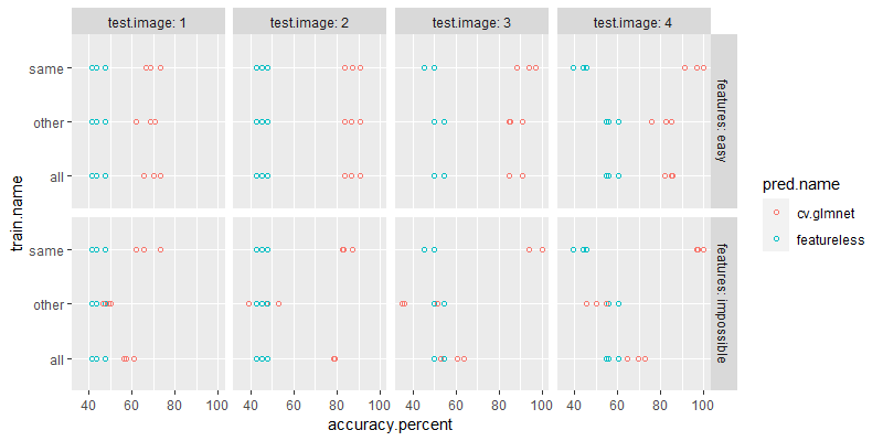
The output above shows the result table with test accuracy for each test fold, test image, train set, feature set, and algorithm. Below we plot these results.
ggplot()+
  geom_point(aes(
    accuracy.percent, train.name, color=pred.name),
    shape=1,
    data=my.score.dt)+
  facet_grid(features ~ test.image, labeller=label_both)
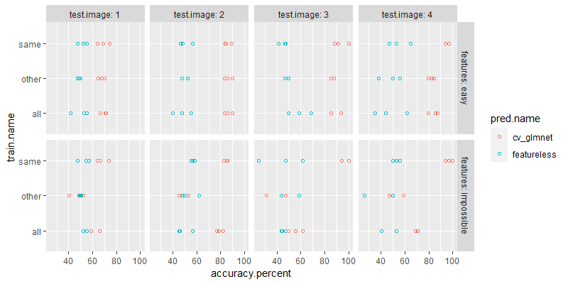
The plot above shows a result which is very similar to what we observed above, using the for loop/future/ResamplingCustom. But we have moved the split logic to a new class, which makes the user code much simpler. All the user has to define in this framework are two lists: data sets and algorithms.
Conclusion
I have shown various R coding techniques which can be used to code
cross-validation, for quantifying the extent to which models can
generalize/predict on new groups. Whereas this is possible but
somewhat complex to code using existing techniques, I have proposed a
new MyResampling class which works with the mlr3 framework, and
greatly simplifies the code necessary for this kind of computational
experiment. For future work, I plan to move this new code to an R
package, published on CRAN, to make these methods easier to implement
for non-experts.
UPDATE Dec 2023: mlr3resampling::ResamplingSameOtherCV is now on CRAN, see ?score for an example.
Session/version info
sessionInfo()
## R version 4.3.2 (2023-10-31 ucrt)
## Platform: x86_64-w64-mingw32/x64 (64-bit)
## Running under: Windows 10 x64 (build 19045)
##
## Matrix products: default
##
##
## locale:
## [1] LC_COLLATE=English_United States.utf8  LC_CTYPE=English_United States.utf8    LC_MONETARY=English_United States.utf8
## [4] LC_NUMERIC=C                           LC_TIME=English_United States.utf8
##
## time zone: America/Phoenix
## tzcode source: internal
##
## attached base packages:
## [1] stats     graphics  grDevices utils     datasets  methods   base
##
## other attached packages:
## [1] ggplot2_3.4.4      data.table_1.14.99
##
## loaded via a namespace (and not attached):
##  [1] utf8_1.2.4           future_1.33.0        generics_0.1.3       shape_1.4.6          lattice_0.22-5
##  [6] listenv_0.9.0        digest_0.6.33        magrittr_2.0.3       evaluate_0.23        grid_4.3.2
## [11] iterators_1.0.14     foreach_1.5.2        glmnet_4.1-8         Matrix_1.6-4         backports_1.4.1
## [16] mlr3learners_0.5.7   survival_3.5-7       fansi_1.0.6          scales_1.3.0         mlr3_0.17.0
## [21] mlr3measures_0.5.0   codetools_0.2-19     palmerpenguins_0.1.1 cli_3.6.2            rlang_1.1.2
## [26] crayon_1.5.2         parallelly_1.36.0    future.apply_1.11.0  munsell_0.5.0        splines_4.3.2
## [31] withr_2.5.2          tools_4.3.2          parallel_4.3.2       uuid_1.1-1           checkmate_2.3.1
## [36] dplyr_1.1.4          colorspace_2.1-0     globals_0.16.2       vctrs_0.6.5          R6_2.5.1
## [41] lifecycle_1.0.4      mlr3misc_0.13.0      pkgconfig_2.0.3      pillar_1.9.0         gtable_0.3.4
## [46] glue_1.6.2           Rcpp_1.0.11          lgr_0.4.4            paradox_0.11.1       xfun_0.41
## [51] tibble_3.2.1         tidyselect_1.2.0     highr_0.10           knitr_1.45           farver_2.1.1
## [56] labeling_0.4.3       compiler_4.3.2