Easily add direct labels to plots using the directlabels package!
 |
This package is an attempt to make direct labeling a reality in
everyday statistical practice by making available a body of useful
functions that make direct labeling of common plots easy to do with
high-level plotting systems such as lattice and ggplot2. The main
function that the package provides is direct.label(p), which
takes a lattice or ggplot2 plot p and adds direct labels:
install.packages("directlabels")
library(lattice)
library(directlabels)
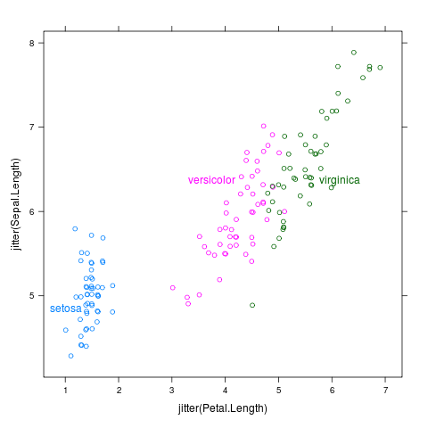
direct.label(xyplot(jitter(Sepal.Length)~jitter(Petal.Length),iris,groups=Species))
directlabels website navigation
Frequently asked questions
- Before
emailing me, please search and post on stackoverflow.
- How to avoid overlapping labels? Use a Positioning Method
with calc.boxes
to compute the label bounding box. For
example, smart.grid
for scatterplots
and last.polygons
or last.qp
for lineplots.
- Can I increase text size? Yes, but do it before calling
Positioning Methods that calculate the label bounding
box: direct.label(p, list(cex=2, "last.qp")) for a lineplot p.
- Why are some labels small when using lineplot labeling methods
like last.polygons?
Because the labels are automatically resized to fit in the plotting
area. To increase the text size you can increase the x axis limits as in
the lars
and ridge
examples.
- How to adjust all labels left or right? For example you can
use direct.label(p, list(dl.trans(x=x+0.1), "last.qp")) to
move labels to the right 0.1cm and then
apply last.qp
for a lineplot p.
- How
about fontface, fontfamily, rot, alpha
text parameters? See example(dlcompare).
- How about direct labeling aesthetics other than colour in ggplot2?
See example(geom_dl).
- Can I use directlabels to label individual points on scatterplots?
The intended purpose of directlabels is to replace a confusing legend
(which labels groups of points, not individual points). You may want
to try to write your own Positioning
Method but be aware
that automatic
label placement is an NP-hard problem!
|
Positioning Methods specify the direct label positions
Direct labeling a plot can be decomposed into 2 steps: calculating
label positions, then drawing the labels. For the first step, the
directlabels package introduces the concept of the Positioning Method,
which is a list that specifies how to transform the data points into
labels. For example, with the scatterplot above, the default
Positioning Method is
smart.grid,
which places each label close to the center of the corresponding point
cloud. The following diagram shows how the data to plot is converted
to standard form column names and positions in centimeters before the
Positioning Method is applied:
Petal.Length Sepal.Length Species
         1.4          5.1  setosa
         1.4          4.9  setosa
         1.3          4.7  setosa
         1.5          4.6  setosa
         1.4          5.0  setosa
         1.7          5.4  setosa
         ...          ...    ...
|
 convert to
 standard form (cm)
--------------------->
 direct.label.trellis
 and
 drawDetails.dlgrob
|
       x        y groups
2.021041 3.786670 setosa
2.021041 3.066771 setosa
1.772450 2.346872 setosa
2.269632 1.986922 setosa
2.021041 3.426721 setosa
2.766813 4.866519 setosa
    ...      ...    ...
|
 calculate label
 positions with
 Positioning Method
--------------------->
 smart.grid
|
         x      y     groups
 0.8364451  3.806     setosa
11.2194634 11.418  virginica
 8.0289573  7.958 versicolor
|
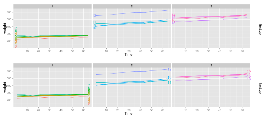
If default label positions are not satisfactory, you can always
specify your own Positioning Method, using the method=
argument to direct.label. For example, we can label
longitudinal data either on the left or right of the lines:
install.packages("ggplot2")
library(ggplot2)
data(BodyWeight,package="nlme")
p <- qplot(Time,weight,data=BodyWeight,colour=Rat,geom="line",facets=.~Diet)
direct.label(p,"first.qp")
direct.label(p,"last.qp")
first.qp and last.qp are the names of Positioning
Methods which place the labels respectively near the first or last
points, ensuring that the labels do not overlap and so are
readable. To find out which built-in Positioning Methods are
appropriate for your plot, check out the
Positioning Methods example database.
However, the power of the directlabels system is the fact that you
can write your own Positioning Methods,
and they can be reused for different plots. So once you write a
Positioning Method that works, adding direct labels in everyday plots
is as simple as calling direct.label, no matter if you are
using lattice or ggplot2.
Talks, links, etc.
Recent
advances in direct labeled graphics
[source]. Invited talk
for semin-r, the Paris R user group (2012).
Adding direct
labels to
plots, Best
Student Poster at useR 2011, attempts to motivate the package and
explain how it works
[source]. Notably,
the "Optimal Labels" section is basically the only documentation of
how to implement
the qp.labels
Positioning Method. The details of the "Modular package design"
section have changed in version 2.0. Rather than
calling label.positions the first time the plot
is printed, we now draw a dlgrob
whose drawDetails method calculates label positions every
time the plot window is resized/redrawn.
semin-r, 15 oct
2009. "Visualizing
multivariate data using lattice and direct labels"
with R code examples. Note
that the latticedl package used in these slides is obsolete,
so please use the directlabels package instead.
Blog reviews: learnr 2010,
Karl
Broman 2011.
The labcurve
function in the Hmisc package provides some similar functionality.
Some notes on extending ggplot2
using custom grid grobs.
More examples
of directlabels
on the R Graphical Manual.
Return to
the GitHub
repository.