directlabels - lineplot - Positioning Method - last.points

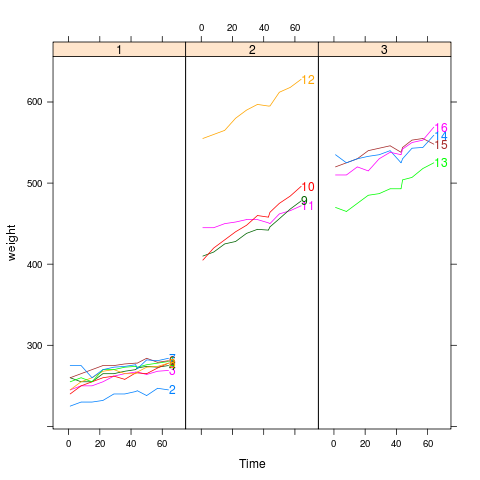bodyweight

data(BodyWeight,package="nlme")
library(lattice)
p <- xyplot(weight~Time|Diet,BodyWeight,groups=Rat,type='l',
       layout=c(3,1),xlim=c(-10,75))
direct.label(p,"last.points")
  

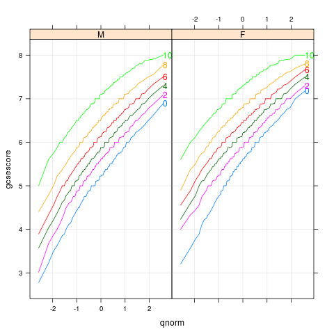chemqqmathscore

data(Chem97,package="mlmRev")
library(lattice)
p <- qqmath(~gcsescore|gender,Chem97,groups=factor(score),
       type=c('l','g'),f.value=ppoints(100))
direct.label(p,"last.points")
  

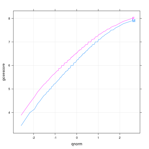chemqqmathsex

data(Chem97,package="mlmRev")
library(lattice)
p <- qqmath(~gcsescore,Chem97,groups=gender,
       type=c("l","g"),f.value=ppoints(100))
direct.label(p,"last.points")
  

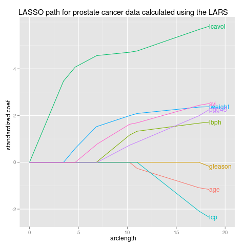lars

data(prostate,package="ElemStatLearn")
pros <- subset(prostate,select=-train,train==TRUE)
ycol <- which(names(pros)=="lpsa")
x <- as.matrix(pros[-ycol])
y <- pros[[ycol]]
library(lars)
fit <- lars(x,y,type="lasso")
beta <- scale(coef(fit),FALSE,1/fit$normx)
arclength <- rowSums(abs(beta))
library(reshape2)
path <- data.frame(melt(beta),arclength)
names(path)[1:3] <- c("step","variable","standardized.coef")
library(ggplot2)
p <- ggplot(path,aes(arclength,standardized.coef,colour=variable))+
  geom_line(aes(group=variable))+
  ggtitle("LASSO path for prostate cancer data calculated using the LARS")+
  xlim(0,20)
direct.label(p,"last.points")
  

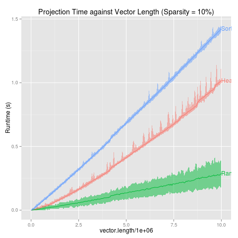projectionSeconds

data(projectionSeconds, package="directlabels")
p <- ggplot(projectionSeconds, aes(vector.length/1e6))+
  geom_ribbon(aes(ymin=min, ymax=max,
                  fill=method, group=method), alpha=1/2)+
  geom_line(aes(y=mean, group=method, colour=method))+
  ggtitle("Projection Time against Vector Length (Sparsity = 10%)")+
  guides(fill="none")+
  ylab("Runtime (s)")
direct.label(p,"last.points")
  

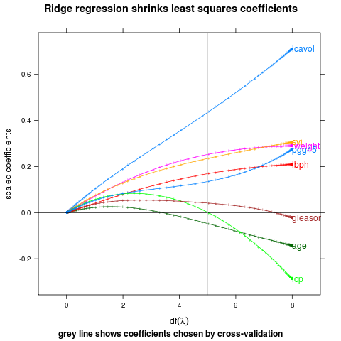ridge

## complicated ridge regression lineplot ex. fig 3.8 from Elements of
## Statistical Learning, Hastie et al.
myridge <- function(f,data,lambda=c(exp(-seq(-15,15,l=200)),0)){
  require(MASS)
  require(reshape2)
  fit <- lm.ridge(f,data,lambda=lambda)
  X <- data[-which(names(data)==as.character(f[[2]]))]
  Xs <- svd(scale(X)) ## my d's should come from the scaled matrix
  dsq <- Xs$d^2
  ## make the x axis degrees of freedom
  df <- sapply(lambda,function(l)sum(dsq/(dsq+l)))
  D <- data.frame(t(fit$coef),lambda,df) # scaled coefs
  molt <- melt(D,id=c("lambda","df"))
  ## add in the points for df=0
  limpts <- transform(subset(molt,lambda==0),lambda=Inf,df=0,value=0)
  rbind(limpts,molt)
}
data(prostate,package="ElemStatLearn")
pros <- subset(prostate,train==TRUE,select=-train)
m <- myridge(lpsa~.,pros)
library(lattice)
p <- xyplot(value~df,m,groups=variable,type="o",pch="+",
       panel=function(...){
         panel.xyplot(...)
         panel.abline(h=0)
         panel.abline(v=5,col="grey")
       },
       xlim=c(-1,9),
       main="Ridge regression shrinks least squares coefficients",
       ylab="scaled coefficients",
       sub="grey line shows coefficients chosen by cross-validation",
       xlab=expression(df(lambda)))
direct.label(p,"last.points")
  

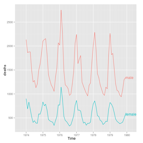sexdeaths

library(ggplot2)
tx <- time(mdeaths)
Time <- ISOdate(floor(tx),round(tx%%1 * 12)+1,1,0,0,0)
uk.lung <- rbind(data.frame(Time,sex="male",deaths=as.integer(mdeaths)),
                 data.frame(Time,sex="female",deaths=as.integer(fdeaths)))
p <- qplot(Time,deaths,data=uk.lung,colour=sex,geom="line")+
  xlim(ISOdate(1973,9,1),ISOdate(1980,4,1))
direct.label(p,"last.points")