More precise imbalanced data generation
The purpose of this page is to continue the exploration of Creating large imbalanced data benchmarks.
Problem
We are creating machine learning algorithms for imbalanced classification problems.
We would like to know if these algorithms work well for training on imbalanced data, and predicting on balanced data, and vice versa.
We therefore would like to create different subsets for testing.
Assume we start with the higgs data, binary classification with this many data in each class:
Tpos=5829123
Tneg=5170877
Below are the target proportions of the minority negative class:
Target_prop <- 10^seq(-1, -5)
Below we repeat the calculations in the previous post:
library(data.table)
(orig_dt <- data.table(
  Target_prop,
  N_pos_neg = as.integer(Tpos/(3-2*Target_prop))
)[
, n_pos := Tpos-N_pos_neg
][
, n_neg := as.integer(Target_prop*n_pos/(1-Target_prop))
][
, n_imb := n_pos+n_neg
][, let(
  pos=n_pos+N_pos_neg,
  neg=n_neg+N_pos_neg,
  check_prop = n_neg/n_imb
)][])
##    Target_prop N_pos_neg   n_pos  n_neg   n_imb     pos     neg   check_prop
##          <num>     <int>   <num>  <int>   <num>   <num>   <int>        <num>
## 1:       1e-01   2081829 3747294 416366 4163660 5829123 2498195 1.000000e-01
## 2:       1e-02   1956081 3873042  39121 3912163 5829123 1995202 9.999839e-03
## 3:       1e-03   1944337 3884786   3888 3888674 5829123 1948225 9.998267e-04
## 4:       1e-04   1943170 3885953    388 3886341 5829123 1943558 9.983684e-05
## 5:       1e-05   1943053 3886070     38 3886108 5829123 1943091 9.778421e-06
The numbers above seem reasonable, but
Target_prop=5e-01(balanced) hasneg>Tnegwhich is not possible (not enough negative samples).- the
Target_prop(desired imbalance) is often a bit larger thancheck_prop(actual imbalance). - the
check_Ncolumns are off by one or two.
Proposed fix
To fix the issues above, we start with the idea that for any target proportion, we want n_neg to be the largest integer such that the number of positive samples used is less than or equal the total number of samples: N + n_pos <= Tpos (and same for negative).
That gives us the code below, which also works for negative proportions greater than 0.5:
compute_target_counts <- function(p_neg, Tpos, Tneg){
  p_small <- ifelse(p_neg<0.5, p_neg, 1-p_neg)
  n_small = as.integer(pmin(
    2*Tpos*p_small/(3*(1-p_neg)+p_neg),
    2*Tneg*p_small/(1+2*p_neg)
  ))
  data.table(p_neg)[, let(
    n_pos = ifelse(
      p_neg<0.5,
      n_small*(1-p_neg)/p_neg,
      n_small),
    n_neg = ifelse(
      p_neg<0.5,
      n_small,
      n_small*p_neg/(1-p_neg))
  )][
  , n_imb := n_pos+n_neg
  ][
  , N_pos := n_imb/2
  ][
  , N_neg := n_imb-N_pos
  ][, let(
    pos=n_pos+N_pos,
    neg=n_neg+N_neg
  )][
  , check_prop := n_neg/n_imb
  ][]
}
p_neg <- sort(c(Target_prop, 1-Target_prop), decreasing = TRUE)
#p_neg <- sort(seq(0.45, 0.55, by=0.01), decreasing = TRUE)
compute_target_counts(p_neg, Tpos, Tneg)
##       p_neg   n_pos   n_neg   n_imb   N_pos   N_neg     pos     neg check_prop
##       <num>   <num>   <num>   <num>   <num>   <num>   <num>   <num>      <num>
##  1: 0.99999      34 3399966 3400000 1700000 1700000 1700034 5099966    0.99999
##  2: 0.99990     344 3439656 3440000 1720000 1720000 1720344 5159656    0.99990
##  3: 0.99900    3449 3445551 3449000 1724500 1724500 1727949 5170051    0.99900
##  4: 0.99000   34703 3435597 3470300 1735150 1735150 1769853 5170747    0.99000
##  5: 0.90000  369348 3324132 3693480 1846740 1846740 2216088 5170872    0.90000
##  6: 0.10000 3747285  416365 4163650 2081825 2081825 5829110 2498190    0.10000
##  7: 0.01000 3872979   39121 3912100 1956050 1956050 5829029 1995171    0.01000
##  8: 0.00100 3884112    3888 3888000 1944000 1944000 5828112 1947888    0.00100
##  9: 0.00010 3879612     388 3880000 1940000 1940000 5819612 1940388    0.00010
## 10: 0.00001 3799962      38 3800000 1900000 1900000 5699962 1900038    0.00001
Visualization
br <- c(10^seq(-5, -1), 0.5)
breaks=unique(c(br, 1-br))
p_lo <- c(
  seq(0.01, 0.5, by=0.01),
  10^seq(-5, -1, by=0.1))
p_grid <- unique(sort(c(p_lo, 1-p_lo)))
(grid_dt <- compute_target_counts(p_grid, Tpos, Tneg))
##             p_neg   n_pos   n_neg   n_imb   N_pos   N_neg     pos     neg   check_prop
##             <num>   <num>   <num>   <num>   <num>   <num>   <num>   <num>        <num>
##   1: 1.000000e-05 3799962      38 3800000 1900000 1900000 5699962 1900038 1.000000e-05
##   2: 1.258925e-05 3812728      48 3812776 1906388 1906388 5719115 1906436 1.258925e-05
##   3: 1.584893e-05 3848779      61 3848840 1924420 1924420 5773199 1924481 1.584893e-05
##   4: 1.995262e-05 3859065      77 3859142 1929571 1929571 5788636 1929648 1.995262e-05
##   5: 2.511886e-05 3861543      97 3861640 1930820 1930820 5792362 1930917 2.511886e-05
##  ---
## 174: 9.999749e-01      86 3423636 3423722 1711861 1711861 1711947 5135497 9.999749e-01
## 175: 9.999800e-01      68 3408005 3408073 1704037 1704037 1704105 5112042 9.999800e-01
## 176: 9.999842e-01      54 3407116 3407170 1703585 1703585 1703639 5110700 9.999842e-01
## 177: 9.999874e-01      43 3415568 3415611 1707806 1707806 1707849 5123374 9.999874e-01
## 178: 9.999900e-01      34 3399966 3400000 1700000 1700000 1700034 5099966 9.999900e-01
grid_dt[, diff := p_neg-check_prop][order(abs(diff))]
##             p_neg   n_pos   n_neg   n_imb   N_pos   N_neg     pos     neg   check_prop          diff
##             <num>   <num>   <num>   <num>   <num>   <num>   <num>   <num>        <num>         <num>
##   1: 1.000000e-05 3799962      38 3800000 1900000 1900000 5699962 1900038 1.000000e-05  0.000000e+00
##   2: 1.584893e-05 3848779      61 3848840 1924420 1924420 5773199 1924481 1.584893e-05  0.000000e+00
##   3: 1.995262e-05 3859065      77 3859142 1929571 1929571 5788636 1929648 1.995262e-05  0.000000e+00
##   4: 2.511886e-05 3861543      97 3861640 1930820 1930820 5792362 1930917 2.511886e-05  0.000000e+00
##   5: 3.981072e-05 3868151     154 3868305 1934153 1934153 5802304 1934307 3.981072e-05  0.000000e+00
##  ---
## 174: 6.400000e-01 1632908 2902948 4535856 2267928 2267928 3900836 5170875 6.400000e-01 -1.110223e-16
## 175: 6.700000e-01 1458452 2961100 4419552 2209776 2209776 3668228 5170875 6.700000e-01 -1.110223e-16
## 176: 6.900000e-01 1347035 2998239 4345274 2172637 2172637 3519672 5170876 6.900000e-01  1.110223e-16
## 177: 7.000000e-01 1292719 3016344 4309063 2154532 2154532 3447251 5170876 7.000000e-01 -1.110223e-16
## 178: 7.100000e-01 1239301 3034151 4273452 2136726 2136726 3376027 5170877 7.100000e-01 -1.110223e-16
library(ggplot2)
(grid_long <- melt(grid_dt, measure.vars=measure(prefix, class, pattern="^(|n_|N_)(pos|neg)$")))
##              p_neg   n_imb   check_prop          diff prefix  class   value
##              <num>   <num>        <num>         <num> <char> <char>   <num>
##    1: 1.000000e-05 3800000 1.000000e-05  0.000000e+00     n_    pos 3799962
##    2: 1.258925e-05 3812776 1.258925e-05 -1.694066e-21     n_    pos 3812728
##    3: 1.584893e-05 3848840 1.584893e-05  0.000000e+00     n_    pos 3848779
##    4: 1.995262e-05 3859142 1.995262e-05  0.000000e+00     n_    pos 3859065
##    5: 2.511886e-05 3861640 2.511886e-05  0.000000e+00     n_    pos 3861543
##   ---
## 1064: 9.999749e-01 3423722 9.999749e-01  0.000000e+00           neg 5135497
## 1065: 9.999800e-01 3408073 9.999800e-01  0.000000e+00           neg 5112042
## 1066: 9.999842e-01 3407170 9.999842e-01  0.000000e+00           neg 5110700
## 1067: 9.999874e-01 3415611 9.999874e-01  0.000000e+00           neg 5123374
## 1068: 9.999900e-01 3400000 9.999900e-01  0.000000e+00           neg 5099966
n_max <- grid_long[, .SD[value==max(value)], by=.(prefix, class)]
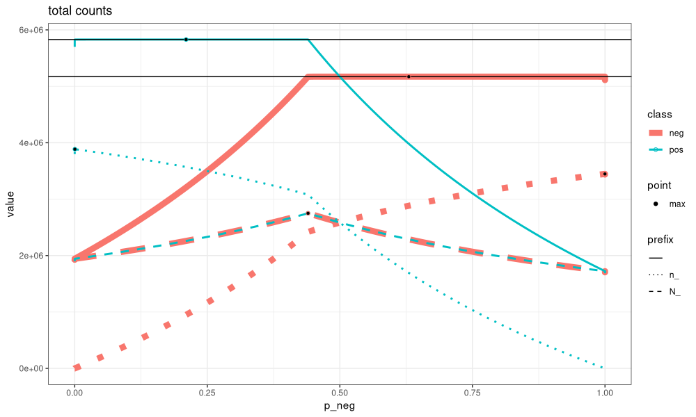
(gg <- ggplot()+
ggtitle("total counts")+
theme_bw()+
scale_size_manual(values=c(
neg=3, pos=1))+
scale_linetype_manual(values=c(
"solid",
"dotted",
"dashed"))+
geom_line(aes(
p_neg, value, color=class, size=class, linetype=prefix),
data=grid_long)+
geom_hline(aes(
yintercept=value),
data=data.frame(value=c(Tpos, Tneg)))+
scale_fill_manual(values=c(max="black"))+
geom_point(aes(
p_neg, value, color=class, fill=point),
shape=21,
data=n_max[, point := "max"]))
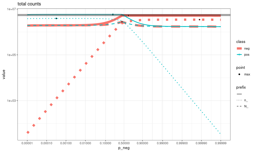
gg+
  scale_x_continuous(transform="logit", breaks=breaks)+
  scale_y_log10()
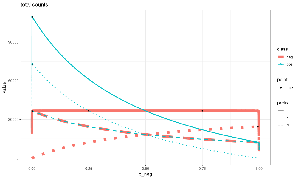
other data
Laribi_dt <- fread("~/projects/stratified-group-cv/data/Laribi2024.csv")
ltab <- table(Laribi_dt$target)
(Laribi_grid_dt <- compute_target_counts(p_grid, ltab[1], ltab[2])[is.finite(check_prop)])
##             p_neg    n_pos    n_neg    n_imb     N_pos     N_neg       pos      neg   check_prop
##             <num>    <num>    <num>    <num>     <num>     <num>     <num>    <num>        <num>
##   1: 1.584893e-05 63094.73     1.00 63095.73 31547.867 31547.867 94642.602 31548.87 1.584893e-05
##   2: 1.995262e-05 50117.72     1.00 50118.72 25059.362 25059.362 75177.085 25060.36 1.995262e-05
##   3: 2.511886e-05 39809.72     1.00 39810.72 19905.359 19905.359 59715.076 19906.36 2.511886e-05
##   4: 3.162278e-05 63243.55     2.00 63245.55 31622.777 31622.777 94866.330 31624.78 3.162278e-05
##   5: 3.981072e-05 50235.73     2.00 50237.73 25118.864 25118.864 75354.593 25120.86 3.981072e-05
##  ---
## 165: 9.998741e-01     3.00 23826.85 23829.85 11914.924 11914.924 11917.924 35741.77 9.998741e-01
## 166: 9.999000e-01     2.00 19998.00 20000.00 10000.000 10000.000 10002.000 29998.00 9.999000e-01
## 167: 9.999206e-01     1.00 12588.25 12589.25  6294.627  6294.627  6295.627 18882.88 9.999206e-01
## 168: 9.999369e-01     1.00 15847.93 15848.93  7924.466  7924.466  7925.466 23772.40 9.999369e-01
## 169: 9.999499e-01     1.00 19951.62 19952.62  9976.312  9976.312  9977.312 29927.93 9.999499e-01
Laribi_grid_dt[, diff := p_neg-check_prop][order(abs(diff))]
##             p_neg    n_pos    n_neg    n_imb    N_pos    N_neg      pos      neg   check_prop          diff
##             <num>    <num>    <num>    <num>    <num>    <num>    <num>    <num>        <num>         <num>
##   1: 1.584893e-05 63094.73     1.00 63095.73 31547.87 31547.87 94642.60 31548.87 1.584893e-05  0.000000e+00
##   2: 1.995262e-05 50117.72     1.00 50118.72 25059.36 25059.36 75177.09 25060.36 1.995262e-05  0.000000e+00
##   3: 2.511886e-05 39809.72     1.00 39810.72 19905.36 19905.36 59715.08 19906.36 2.511886e-05  0.000000e+00
##   4: 3.162278e-05 63243.55     2.00 63245.55 31622.78 31622.78 94866.33 31624.78 3.162278e-05  0.000000e+00
##   5: 3.981072e-05 50235.73     2.00 50237.73 25118.86 25118.86 75354.59 25120.86 3.981072e-05  0.000000e+00
##  ---
## 165: 3.700000e-01 26579.19 15610.00 42189.19 21094.59 21094.59 47673.78 36704.59 3.700000e-01 -5.551115e-17
## 166: 4.400000e-01 21866.73 17181.00 39047.73 19523.86 19523.86 41390.59 36704.86 4.400000e-01  5.551115e-17
## 167: 4.600000e-01 20645.61 17587.00 38232.61 19116.30 19116.30 39761.91 36703.30 4.600000e-01  5.551115e-17
## 168: 4.500000e-01 21249.56 17386.00 38635.56 19317.78 19317.78 40567.33 36703.78 4.500000e-01  1.110223e-16
## 169: 5.500000e-01 15730.00 19225.56 34955.56 17477.78 17477.78 33207.78 36703.33 5.500000e-01  1.110223e-16
(grid_long <- melt(Laribi_grid_dt, measure.vars=measure(prefix, class, pattern="^(|n_|N_)(pos|neg)$")))
##              p_neg    n_imb   check_prop  diff prefix  class    value
##              <num>    <num>        <num> <num> <char> <char>    <num>
##    1: 1.584893e-05 63095.73 1.584893e-05     0     n_    pos 63094.73
##    2: 1.995262e-05 50118.72 1.995262e-05     0     n_    pos 50117.72
##    3: 2.511886e-05 39810.72 2.511886e-05     0     n_    pos 39809.72
##    4: 3.162278e-05 63245.55 3.162278e-05     0     n_    pos 63243.55
##    5: 3.981072e-05 50237.73 3.981072e-05     0     n_    pos 50235.73
##   ---
## 1010: 9.998741e-01 23829.85 9.998741e-01     0           neg 35741.77
## 1011: 9.999000e-01 20000.00 9.999000e-01     0           neg 29998.00
## 1012: 9.999206e-01 12589.25 9.999206e-01     0           neg 18882.88
## 1013: 9.999369e-01 15848.93 9.999369e-01     0           neg 23772.40
## 1014: 9.999499e-01 19952.62 9.999499e-01     0           neg 29927.93
n_max <- grid_long[, .SD[value==max(value)], by=.(prefix, class)]

(gg <- ggplot()+
   ggtitle("total counts")+
   theme_bw()+
   scale_size_manual(values=c(
     neg=3, pos=1))+
   scale_linetype_manual(values=c(
     "solid",
     "dotted",
     "dashed"))+
   geom_line(aes(
     p_neg, value, color=class, size=class, linetype=prefix),
     data=grid_long)+
   scale_fill_manual(values=c(max="black"))+
   geom_point(aes(
     p_neg, value, color=class, fill=point),
     shape=21,
     data=n_max[, point := "max"]))
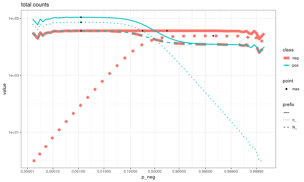
gg+
  scale_x_continuous(transform="logit", breaks=breaks)+
  scale_y_log10()
session info
sessionInfo()
## R version 4.5.3 (2026-03-11)
## Platform: x86_64-pc-linux-gnu
## Running under: Ubuntu 24.04.4 LTS
##
## Matrix products: default
## BLAS:   /usr/lib/x86_64-linux-gnu/blas/libblas.so.3.12.0
## LAPACK: /usr/lib/x86_64-linux-gnu/lapack/liblapack.so.3.12.0  LAPACK version 3.12.0
##
## locale:
##  [1] LC_CTYPE=en_US.UTF-8       LC_NUMERIC=C               LC_TIME=fr_FR.UTF-8        LC_COLLATE=en_US.UTF-8
##  [5] LC_MONETARY=fr_FR.UTF-8    LC_MESSAGES=en_US.UTF-8    LC_PAPER=fr_FR.UTF-8       LC_NAME=C
##  [9] LC_ADDRESS=C               LC_TELEPHONE=C             LC_MEASUREMENT=fr_FR.UTF-8 LC_IDENTIFICATION=C
##
## time zone: America/Toronto
## tzcode source: system (glibc)
##
## attached base packages:
## [1] stats     graphics  grDevices utils     datasets  methods   base
##
## other attached packages:
## [1] ggplot2_4.0.3     data.table_1.18.4
##
## loaded via a namespace (and not attached):
##  [1] vctrs_0.7.3        cli_3.6.6          knitr_1.51         rlang_1.2.0        xfun_0.57          otel_0.2.0
##  [7] generics_0.1.4     S7_0.2.2           glue_1.8.1         labeling_0.4.3     nc_2026.4.20       scales_1.4.0
## [13] grid_4.5.3         evaluate_1.0.5     tibble_3.3.1       lifecycle_1.0.5    compiler_4.5.3     dplyr_1.2.1
## [19] RColorBrewer_1.1-3 pkgconfig_2.0.3    farver_2.1.2       R6_2.6.1           tidyselect_1.2.1   pillar_1.11.1
## [25] magrittr_2.0.5     tools_4.5.3        withr_3.0.2        gtable_0.3.6