Volcano plots
The goal of this post is to describe a similarity between volcano plots and the SOAK summary plots that appear in our recent paper, SOAK: Same/Other/All K-fold cross-validation for estimating similarity of patterns in data subsets, arXiv:2410.08643.
Volcano plot
Volcano plots are a classic representation of effect size and statistical significance, when doing differential expression analysis in genomic data. For example, the sanssouci github repo has the volcano plot below:
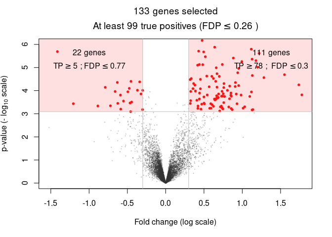
Each dot in the volcano plot represents a different gene. The genes which appear at the bottom center have little difference between groups. The genes which appear in the upper left or right have significant differences between groups.
SOAK plot
The slides for presenting my SOAK paper have the plot below:
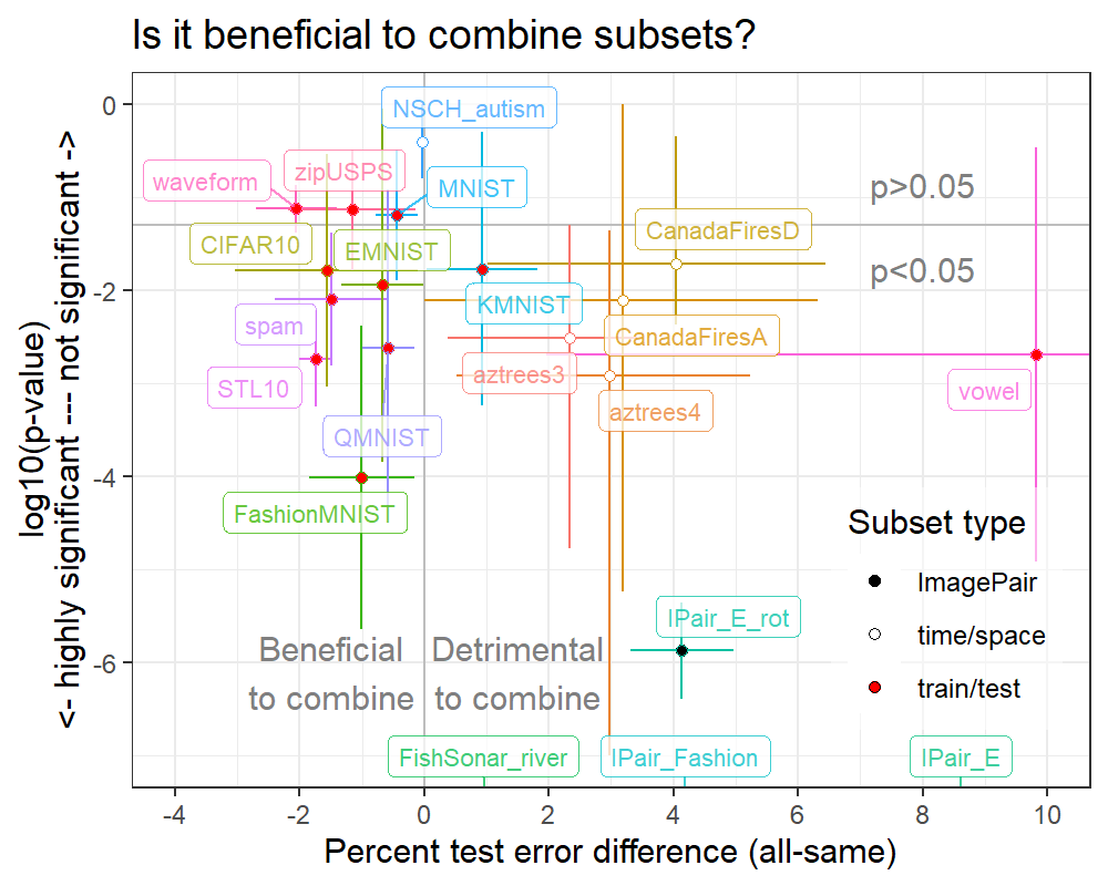
Each dot in the plot above represents one of twenty data sets that we analyzed using SOAK. The line segments represent the range of differences and p-values observed across the 2-4 data subsets. The typical V shape is not apparent because:
- The Y axis in inverted with respect to the volcano plot, and
- The line segments are useful to summarize each data set, but hide the details about the value of each data subset.
Re-making the SOAK plot like a volcano plot
data.list <- list()
local.csv.vec <- c("data-meta.csv", "data_Classif_batchmark_registry.csv")
prefix <- "https://raw.githubusercontent.com/tdhock/cv-same-other-paper/refs/heads/main/"
for(local.csv in local.csv.vec){
  if(!file.exists(local.csv)){
    u <- paste0(prefix, local.csv)
    download.file(u, local.csv)
  }
  data.list[[local.csv]] <- fread(local.csv)
}
library(data.table)
(score.atomic <- data.list$data_Class[, .(
  data.name,
  test_subset = test.group,
  train_subsets = train.groups,
  test.fold, task_id, algorithm, percent.error
)])
##       data.name test_subset train_subsets test.fold  task_id   algorithm percent.error
##          <char>      <char>        <char>     <int>   <char>      <char>         <num>
##    1:  aztrees3          NE           all         1 aztrees3   cv_glmnet      0.000000
##    2:  aztrees3          NW           all         1 aztrees3   cv_glmnet      1.910828
##    3:  aztrees3           S           all         1 aztrees3   cv_glmnet      4.095563
##    4:  aztrees3          NE           all         2 aztrees3   cv_glmnet      4.081633
##    5:  aztrees3          NW           all         2 aztrees3   cv_glmnet      1.910828
##   ---
## 2932:   zipUSPS       train          same         8  zipUSPS featureless     83.608815
## 2933:   zipUSPS        test          same         9  zipUSPS featureless     81.725888
## 2934:   zipUSPS       train          same         9  zipUSPS featureless     83.586207
## 2935:   zipUSPS        test          same        10  zipUSPS featureless     82.142857
## 2936:   zipUSPS       train          same        10  zipUSPS featureless     83.586207
The table above contains the results of running SOAK with two
algorithms (cv_glmnet and featureless) on 20 classification data
sets. The percent.error column contains the test error for
predicting on test_subset, after training on train_subsets.
Data <- function(data.name, Data){
  data.table(data.name, Data)
}
disp.dt <- rbind(
  Data("CanadaFires_all","CanadaFiresA"),
  Data("CanadaFires_downSampled","CanadaFiresD"),
  Data("MNIST_EMNIST", "IPair_E"),
  Data("MNIST_EMNIST_rot", "IPair_E_rot"),
  Data("MNIST_FashionMNIST","IPair_Fashion"))
meta.raw <- data.list[["data-meta.csv"]][
  grepl("train|test",group.small.name), `:=`(
    test=ifelse(group.small.name=="test", group.small.N, group.large.N),
    train=ifelse(group.small.name=="train", group.small.N, group.large.N)
  )
][
, `test%` := as.integer(100*test/rows)
][
, subset_type := fcase(
  grepl("MNIST_", data.name), "ImagePair",
  !is.na(test), "train/test",
  default="time/space")
][]
meta.dt <- disp.dt[
  meta.raw, on="data.name"
][is.na(Data), Data := data.name][]
meta.dt[order(subset_type,data.name), .(subset_type, data.name, group.tab)]
##     subset_type               data.name                                   group.tab
##          <char>                  <char>                                      <char>
##  1:   ImagePair            MNIST_EMNIST                    EMNIST=70000;MNIST=70000
##  2:   ImagePair        MNIST_EMNIST_rot                EMNIST_rot=70000;MNIST=70000
##  3:   ImagePair      MNIST_FashionMNIST              FashionMNIST=70000;MNIST=70000
##  4:  time/space         CanadaFires_all           306=364;329=755;395=1170;326=2538
##  5:  time/space CanadaFires_downSampled             306=287;329=304;326=450;395=450
##  6:  time/space         FishSonar_river CHI=638475;PRL=667201;LEA=739745;BOU=770323
##  7:  time/space             NSCH_autism                       2019=18202;2020=27808
##  8:  time/space                aztrees3                      NE=1464;NW=1563;S=2929
##  9:  time/space                aztrees4              SW=497;NE=1464;NW=1563;SE=2432
## 10:  train/test                 CIFAR10                      test=10000;train=50000
## 11:  train/test                  EMNIST                      test=10000;train=60000
## 12:  train/test            FashionMNIST                      test=10000;train=60000
## 13:  train/test                  KMNIST                      test=10000;train=60000
## 14:  train/test                   MNIST                      test=10000;train=60000
## 15:  train/test                  QMNIST                      test=60000;train=60000
## 16:  train/test                   STL10                        train=5000;test=8000
## 17:  train/test                    spam                        test=1536;train=3065
## 18:  train/test                   vowel                          test=462;train=528
## 19:  train/test                waveform                          train=300;test=500
## 20:  train/test                 zipUSPS                        test=2007;train=7291
##     subset_type               data.name                                   group.tab
The table above contains meta-data, one row for each of the twenty data sets analyzed using SOAK. Next, we compute a wide table of percent error values:
group.meta <- meta.dt[, nc::capture_all_str(
  group.tab,
  test_subset="[^;]+",
  "=",
  subset_rows="[0-9]+", as.integer
), by=data.name]
score.join <- meta.dt[score.atomic, on="data.name"]
(tab.wide <- dcast(
  score.join[algorithm=="cv_glmnet"],
  subset_type + Data + test_subset + test.fold ~ train_subsets,
  value.var="percent.error"))
## Key: <subset_type, Data, test_subset, test.fold>
##      subset_type    Data test_subset test.fold       all     other     same
##           <char>  <char>      <char>     <int>     <num>     <num>    <num>
##   1:   ImagePair IPair_E      EMNIST         1 15.228571 81.900000 6.357143
##   2:   ImagePair IPair_E      EMNIST         2 15.914286 81.214286 6.657143
##   3:   ImagePair IPair_E      EMNIST         3 14.842857 81.042857 6.457143
##   4:   ImagePair IPair_E      EMNIST         4 15.442857 80.600000 6.542857
##   5:   ImagePair IPair_E      EMNIST         5 15.728571 80.057143 6.642857
##  ---
## 486:  train/test zipUSPS       train         6  3.988996  6.740028 4.126547
## 487:  train/test zipUSPS       train         7  5.234160  7.988981 4.958678
## 488:  train/test zipUSPS       train         8  5.371901  7.851240 5.647383
## 489:  train/test zipUSPS       train         9  4.413793  8.275862 5.241379
## 490:  train/test zipUSPS       train        10  5.655172  7.862069 6.206897
The table above has one row for each combination of (Data set,
test.fold, test_subset), and one column for each value of
train_subsets (all, other, same). We convert to long form below:
(tab.long.raw <- melt(
  tab.wide,
  measure=c("other","all"),
  variable.name="compare_name",
  value.name="compare_error"))
##      subset_type    Data test_subset test.fold     same compare_name compare_error
##           <char>  <char>      <char>     <int>    <num>       <fctr>         <num>
##   1:   ImagePair IPair_E      EMNIST         1 6.357143        other     81.900000
##   2:   ImagePair IPair_E      EMNIST         2 6.657143        other     81.214286
##   3:   ImagePair IPair_E      EMNIST         3 6.457143        other     81.042857
##   4:   ImagePair IPair_E      EMNIST         4 6.542857        other     80.600000
##   5:   ImagePair IPair_E      EMNIST         5 6.642857        other     80.057143
##  ---
## 976:  train/test zipUSPS       train         6 4.126547          all      3.988996
## 977:  train/test zipUSPS       train         7 4.958678          all      5.234160
## 978:  train/test zipUSPS       train         8 5.647383          all      5.371901
## 979:  train/test zipUSPS       train         9 5.241379          all      4.413793
## 980:  train/test zipUSPS       train        10 6.206897          all      5.655172
The long form above lets us compare same with other and all, using the P-value computation below:
computeP <- function(...){
  by.vec <- c(...)
  tab.long.raw[, {
    test.res <- t.test(compare_error, same, paired=TRUE)
    log.signed.p <- function(signed.p){
      sign(signed.p)*abs(log10(abs(signed.p)))
    }
    with(test.res, data.table(
      estimate,
      p.value,
      compare_mean=mean(compare_error,na.rm=TRUE),
      same_mean=mean(same,na.rm=TRUE),
      log10.p=log10(p.value),
      sign.log.p=log.signed.p(p.value*sign(estimate)),
      N=.N))
  }, by=by.vec]
}
p.each.group <- computeP("subset_type","Data","compare_name","test_subset")
compare.wide.groups <- dcast(
  p.each.group,
  subset_type + Data ~ compare_name,
  list(min, max, mean),
  value.var=c("estimate","log10.p"))
tab.long <- computeP("subset_type","Data","compare_name")
(compare.wide <- dcast(
  tab.long,
  subset_type + Data ~ compare_name,
  value.var=c("estimate","log10.p")
)[compare.wide.groups, on=.(subset_type,Data)])
## Key: <subset_type, Data>
##     subset_type            Data estimate_other estimate_all log10.p_other log10.p_all estimate_min_other
##          <char>          <char>          <num>        <num>         <num>       <num>              <num>
##  1:   ImagePair         IPair_E    73.94278441   8.58414037  -36.12557898 -19.9571317        73.21985454
##  2:   ImagePair     IPair_E_rot    37.78295684   4.13574119  -28.05149106 -10.0273169        36.73305654
##  3:   ImagePair   IPair_Fashion    81.12217939   3.60643915  -26.29380602 -11.1659249        77.52428571
##  4:  time/space    CanadaFiresA    12.73119454   3.19346986  -12.15139280  -4.4954774         2.37373163
##  5:  time/space    CanadaFiresD    11.08297211   4.04950901  -10.55342170  -5.4355425         7.23655914
##  6:  time/space FishSonar_river     2.14222066   1.67869144   -9.46757756  -7.1417503         0.50044287
##  7:  time/space     NSCH_autism     0.06869678  -0.03295173   -0.80281281  -0.5788356        -0.06038222
##  8:  time/space        aztrees3    12.75254188   2.33742877   -4.94136087  -3.9006761         3.32686381
##  9:  time/space        aztrees4    10.91479089   2.97026492   -6.01927681  -4.5729462         3.01043395
## 10:  train/test         CIFAR10     0.06900000  -1.57100000   -0.03427972  -2.5555501        -2.79000000
## 11:  train/test          EMNIST    -0.22719298  -0.70789474   -0.28990449  -2.6439777        -1.49000000
## 12:  train/test    FashionMNIST     0.27250000  -1.00583333   -0.25506863  -3.8370923        -1.62000000
## 13:  train/test          KMNIST     5.73250000   0.93333333  -10.54167700  -2.6079393         4.14000000
## 14:  train/test           MNIST     0.40268174  -0.44128882   -0.71578296  -2.0236324        -0.64938271
## 15:  train/test          QMNIST     0.20330352  -0.58918097   -0.49318750  -3.6638006        -0.59667262
## 16:  train/test           STL10     0.15750000  -1.73750000   -0.10956553  -4.6478898        -1.06000000
## 17:  train/test            spam    -0.68438147  -1.49749989   -0.80213878  -3.3172339        -1.43284293
## 18:  train/test           vowel    28.70454545   9.81818182   -9.42176606  -3.4375486        23.50000000
## 19:  train/test        waveform    -0.60749910  -2.05518719   -0.26171299  -1.5446149        -2.04671858
## 20:  train/test         zipUSPS     0.23993120  -1.16190955   -0.14697286  -1.8158690        -2.08458852
##     subset_type            Data estimate_other estimate_all log10.p_other log10.p_all estimate_min_other
##     estimate_min_all log10.p_min_other log10.p_min_all estimate_max_other estimate_max_all log10.p_max_other
##                <num>             <num>           <num>              <num>            <num>             <num>
##  1:     8.162724e+00       -19.1855428     -11.1852296         74.6657143     9.052381e+00      -18.34494658
##  2:     3.312752e+00       -15.2819271      -6.3918049         38.8328571     4.958730e+00      -15.12765365
##  3:     2.584307e+00       -21.6603229     -12.3831809         84.7200731     4.628571e+00      -17.76668547
##  4:    -2.218278e-17        -6.7029138      -5.2462861         20.5797080     6.321321e+00       -2.42289502
##  5:     1.010753e+00        -3.6935764      -2.3633517         16.0000000     6.444444e+00       -2.52272197
##  6:     4.752551e-01       -14.6703314     -14.3648065          4.6164502     4.364652e+00       -8.14097009
##  7:    -6.589182e-02        -2.8915032      -0.7920586          0.1977758    -1.163559e-05       -0.46373255
##  8:     3.833958e-01        -7.9297112      -4.7714958         30.5950051     3.419998e+00       -2.93905476
##  9:     5.124228e-01        -9.1721995      -7.0049919         29.7819402     5.224490e+00       -1.66564731
## 10:    -3.040000e+00        -7.2308941      -3.0308816          2.9280000    -1.020000e-01       -3.14915524
## 11:    -1.330000e+00        -6.3649830      -3.8468297          1.1759259    -1.666667e-02       -3.70550402
## 12:    -1.850000e+00        -6.2626646      -5.6422445          2.1650000    -1.616667e-01       -4.45852315
## 13:     4.666667e-02       -10.7469910      -3.2389992          7.3250000     1.820000e+00       -5.70697352
## 14:    -7.792532e-01        -3.4218128      -1.8923095          1.4547462    -1.033244e-01       -1.59415295
## 15:    -1.028346e+00        -4.9293022      -4.3218119          1.0032797    -1.500164e-01       -3.31918513
## 16:    -2.000000e+00        -1.6011453      -3.2481787          1.3750000    -1.475000e+00       -0.63846190
## 17:    -2.408148e+00        -1.0340034      -2.8057248          0.0640800    -5.868522e-01       -0.04967194
## 18:     1.954545e+00        -5.4806885      -4.9159399         33.9090909     1.768182e+01       -4.79314130
## 19:    -2.701891e+00        -0.6362025      -1.3740040          0.8317204    -1.408483e+00       -0.33892053
## 20:    -2.185365e+00        -6.7564815      -1.7849263          2.5644509    -1.384545e-01       -1.76993887
##     estimate_min_all log10.p_min_other log10.p_min_all estimate_max_other estimate_max_all log10.p_max_other
##     log10.p_max_all estimate_mean_other estimate_mean_all log10.p_mean_other log10.p_mean_all
##               <num>               <num>             <num>              <num>            <num>
##  1:   -1.019233e+01         73.94278441        8.60755240        -18.7652447      -10.6887780
##  2:   -5.363052e+00         37.78295684        4.13574119        -15.2047904       -5.8774285
##  3:   -8.637530e+00         81.12217939        3.60643915        -19.7135042      -10.5103556
##  4:    0.000000e+00         12.73119454        3.19346986         -5.3215789       -2.1054884
##  5:   -3.372540e-01         11.08297211        4.04950901         -3.0903031       -1.7121430
##  6:   -8.575531e+00          2.14222066        1.67869144        -12.6392296      -11.3247505
##  7:   -1.067407e-04          0.06869678       -0.03295173         -1.6776179       -0.3960826
##  8:   -1.295590e+00         12.75254188        2.33742877         -5.5645877       -2.5108077
##  9:   -1.352162e+00         10.91479089        2.97026492         -4.8362095       -2.9181016
## 10:   -5.324016e-01          0.06900000       -1.57100000         -5.1900247       -1.7816416
## 11:   -4.231388e-02         -0.15703704       -0.67333333         -5.0352435       -1.9445718
## 12:   -2.384369e+00          0.27250000       -1.00583333         -5.3605939       -4.0133067
## 13:   -2.984299e-01          5.73250000        0.93333333         -8.2269822       -1.7687145
## 14:   -4.840571e-01          0.40268174       -0.44128882         -2.5079829       -1.1881833
## 15:   -9.119973e-01          0.20330352       -0.58918097         -4.1242437       -2.6169046
## 16:   -2.216951e+00          0.15750000       -1.73750000         -1.1198036       -2.7325648
## 17:   -1.384153e+00         -0.68438147       -1.49749989         -0.5418377       -2.0949387
## 18:   -4.648515e-01         28.70454545        9.81818182         -5.1369149       -2.6903957
## 19:   -8.655658e-01         -0.60749910       -2.05518719         -0.4875615       -1.1197849
## 20:   -4.823761e-01          0.23993120       -1.16190955         -4.2632102       -1.1336512
##     log10.p_max_all estimate_mean_other estimate_mean_all log10.p_mean_other log10.p_mean_all
The table above has one row per data set, and columns for different statistics (min, max, mean) of P-value (log10.p) and test error difference (estimate). The code below reproduces the SOAK figure.
compare.wide[log10.p_all < -12, log10.p_all := -Inf][]
## Key: <subset_type, Data>
##     subset_type            Data estimate_other estimate_all log10.p_other log10.p_all estimate_min_other
##          <char>          <char>          <num>        <num>         <num>       <num>              <num>
##  1:   ImagePair         IPair_E    73.94278441   8.58414037  -36.12557898        -Inf        73.21985454
##  2:   ImagePair     IPair_E_rot    37.78295684   4.13574119  -28.05149106 -10.0273169        36.73305654
##  3:   ImagePair   IPair_Fashion    81.12217939   3.60643915  -26.29380602 -11.1659249        77.52428571
##  4:  time/space    CanadaFiresA    12.73119454   3.19346986  -12.15139280  -4.4954774         2.37373163
##  5:  time/space    CanadaFiresD    11.08297211   4.04950901  -10.55342170  -5.4355425         7.23655914
##  6:  time/space FishSonar_river     2.14222066   1.67869144   -9.46757756  -7.1417503         0.50044287
##  7:  time/space     NSCH_autism     0.06869678  -0.03295173   -0.80281281  -0.5788356        -0.06038222
##  8:  time/space        aztrees3    12.75254188   2.33742877   -4.94136087  -3.9006761         3.32686381
##  9:  time/space        aztrees4    10.91479089   2.97026492   -6.01927681  -4.5729462         3.01043395
## 10:  train/test         CIFAR10     0.06900000  -1.57100000   -0.03427972  -2.5555501        -2.79000000
## 11:  train/test          EMNIST    -0.22719298  -0.70789474   -0.28990449  -2.6439777        -1.49000000
## 12:  train/test    FashionMNIST     0.27250000  -1.00583333   -0.25506863  -3.8370923        -1.62000000
## 13:  train/test          KMNIST     5.73250000   0.93333333  -10.54167700  -2.6079393         4.14000000
## 14:  train/test           MNIST     0.40268174  -0.44128882   -0.71578296  -2.0236324        -0.64938271
## 15:  train/test          QMNIST     0.20330352  -0.58918097   -0.49318750  -3.6638006        -0.59667262
## 16:  train/test           STL10     0.15750000  -1.73750000   -0.10956553  -4.6478898        -1.06000000
## 17:  train/test            spam    -0.68438147  -1.49749989   -0.80213878  -3.3172339        -1.43284293
## 18:  train/test           vowel    28.70454545   9.81818182   -9.42176606  -3.4375486        23.50000000
## 19:  train/test        waveform    -0.60749910  -2.05518719   -0.26171299  -1.5446149        -2.04671858
## 20:  train/test         zipUSPS     0.23993120  -1.16190955   -0.14697286  -1.8158690        -2.08458852
##     subset_type            Data estimate_other estimate_all log10.p_other log10.p_all estimate_min_other
##     estimate_min_all log10.p_min_other log10.p_min_all estimate_max_other estimate_max_all log10.p_max_other
##                <num>             <num>           <num>              <num>            <num>             <num>
##  1:     8.162724e+00       -19.1855428     -11.1852296         74.6657143     9.052381e+00      -18.34494658
##  2:     3.312752e+00       -15.2819271      -6.3918049         38.8328571     4.958730e+00      -15.12765365
##  3:     2.584307e+00       -21.6603229     -12.3831809         84.7200731     4.628571e+00      -17.76668547
##  4:    -2.218278e-17        -6.7029138      -5.2462861         20.5797080     6.321321e+00       -2.42289502
##  5:     1.010753e+00        -3.6935764      -2.3633517         16.0000000     6.444444e+00       -2.52272197
##  6:     4.752551e-01       -14.6703314     -14.3648065          4.6164502     4.364652e+00       -8.14097009
##  7:    -6.589182e-02        -2.8915032      -0.7920586          0.1977758    -1.163559e-05       -0.46373255
##  8:     3.833958e-01        -7.9297112      -4.7714958         30.5950051     3.419998e+00       -2.93905476
##  9:     5.124228e-01        -9.1721995      -7.0049919         29.7819402     5.224490e+00       -1.66564731
## 10:    -3.040000e+00        -7.2308941      -3.0308816          2.9280000    -1.020000e-01       -3.14915524
## 11:    -1.330000e+00        -6.3649830      -3.8468297          1.1759259    -1.666667e-02       -3.70550402
## 12:    -1.850000e+00        -6.2626646      -5.6422445          2.1650000    -1.616667e-01       -4.45852315
## 13:     4.666667e-02       -10.7469910      -3.2389992          7.3250000     1.820000e+00       -5.70697352
## 14:    -7.792532e-01        -3.4218128      -1.8923095          1.4547462    -1.033244e-01       -1.59415295
## 15:    -1.028346e+00        -4.9293022      -4.3218119          1.0032797    -1.500164e-01       -3.31918513
## 16:    -2.000000e+00        -1.6011453      -3.2481787          1.3750000    -1.475000e+00       -0.63846190
## 17:    -2.408148e+00        -1.0340034      -2.8057248          0.0640800    -5.868522e-01       -0.04967194
## 18:     1.954545e+00        -5.4806885      -4.9159399         33.9090909     1.768182e+01       -4.79314130
## 19:    -2.701891e+00        -0.6362025      -1.3740040          0.8317204    -1.408483e+00       -0.33892053
## 20:    -2.185365e+00        -6.7564815      -1.7849263          2.5644509    -1.384545e-01       -1.76993887
##     estimate_min_all log10.p_min_other log10.p_min_all estimate_max_other estimate_max_all log10.p_max_other
##     log10.p_max_all estimate_mean_other estimate_mean_all log10.p_mean_other log10.p_mean_all
##               <num>               <num>             <num>              <num>            <num>
##  1:   -1.019233e+01         73.94278441        8.60755240        -18.7652447      -10.6887780
##  2:   -5.363052e+00         37.78295684        4.13574119        -15.2047904       -5.8774285
##  3:   -8.637530e+00         81.12217939        3.60643915        -19.7135042      -10.5103556
##  4:    0.000000e+00         12.73119454        3.19346986         -5.3215789       -2.1054884
##  5:   -3.372540e-01         11.08297211        4.04950901         -3.0903031       -1.7121430
##  6:   -8.575531e+00          2.14222066        1.67869144        -12.6392296      -11.3247505
##  7:   -1.067407e-04          0.06869678       -0.03295173         -1.6776179       -0.3960826
##  8:   -1.295590e+00         12.75254188        2.33742877         -5.5645877       -2.5108077
##  9:   -1.352162e+00         10.91479089        2.97026492         -4.8362095       -2.9181016
## 10:   -5.324016e-01          0.06900000       -1.57100000         -5.1900247       -1.7816416
## 11:   -4.231388e-02         -0.15703704       -0.67333333         -5.0352435       -1.9445718
## 12:   -2.384369e+00          0.27250000       -1.00583333         -5.3605939       -4.0133067
## 13:   -2.984299e-01          5.73250000        0.93333333         -8.2269822       -1.7687145
## 14:   -4.840571e-01          0.40268174       -0.44128882         -2.5079829       -1.1881833
## 15:   -9.119973e-01          0.20330352       -0.58918097         -4.1242437       -2.6169046
## 16:   -2.216951e+00          0.15750000       -1.73750000         -1.1198036       -2.7325648
## 17:   -1.384153e+00         -0.68438147       -1.49749989         -0.5418377       -2.0949387
## 18:   -4.648515e-01         28.70454545        9.81818182         -5.1369149       -2.6903957
## 19:   -8.655658e-01         -0.60749910       -2.05518719         -0.4875615       -1.1197849
## 20:   -4.823761e-01          0.23993120       -1.16190955         -4.2632102       -1.1336512
##     log10.p_max_all estimate_mean_other estimate_mean_all log10.p_mean_other log10.p_mean_all
compare.wide[log10.p_other < -20, log10.p_other := -Inf][]
## Key: <subset_type, Data>
##     subset_type            Data estimate_other estimate_all log10.p_other log10.p_all estimate_min_other
##          <char>          <char>          <num>        <num>         <num>       <num>              <num>
##  1:   ImagePair         IPair_E    73.94278441   8.58414037          -Inf        -Inf        73.21985454
##  2:   ImagePair     IPair_E_rot    37.78295684   4.13574119          -Inf -10.0273169        36.73305654
##  3:   ImagePair   IPair_Fashion    81.12217939   3.60643915          -Inf -11.1659249        77.52428571
##  4:  time/space    CanadaFiresA    12.73119454   3.19346986  -12.15139280  -4.4954774         2.37373163
##  5:  time/space    CanadaFiresD    11.08297211   4.04950901  -10.55342170  -5.4355425         7.23655914
##  6:  time/space FishSonar_river     2.14222066   1.67869144   -9.46757756  -7.1417503         0.50044287
##  7:  time/space     NSCH_autism     0.06869678  -0.03295173   -0.80281281  -0.5788356        -0.06038222
##  8:  time/space        aztrees3    12.75254188   2.33742877   -4.94136087  -3.9006761         3.32686381
##  9:  time/space        aztrees4    10.91479089   2.97026492   -6.01927681  -4.5729462         3.01043395
## 10:  train/test         CIFAR10     0.06900000  -1.57100000   -0.03427972  -2.5555501        -2.79000000
## 11:  train/test          EMNIST    -0.22719298  -0.70789474   -0.28990449  -2.6439777        -1.49000000
## 12:  train/test    FashionMNIST     0.27250000  -1.00583333   -0.25506863  -3.8370923        -1.62000000
## 13:  train/test          KMNIST     5.73250000   0.93333333  -10.54167700  -2.6079393         4.14000000
## 14:  train/test           MNIST     0.40268174  -0.44128882   -0.71578296  -2.0236324        -0.64938271
## 15:  train/test          QMNIST     0.20330352  -0.58918097   -0.49318750  -3.6638006        -0.59667262
## 16:  train/test           STL10     0.15750000  -1.73750000   -0.10956553  -4.6478898        -1.06000000
## 17:  train/test            spam    -0.68438147  -1.49749989   -0.80213878  -3.3172339        -1.43284293
## 18:  train/test           vowel    28.70454545   9.81818182   -9.42176606  -3.4375486        23.50000000
## 19:  train/test        waveform    -0.60749910  -2.05518719   -0.26171299  -1.5446149        -2.04671858
## 20:  train/test         zipUSPS     0.23993120  -1.16190955   -0.14697286  -1.8158690        -2.08458852
##     subset_type            Data estimate_other estimate_all log10.p_other log10.p_all estimate_min_other
##     estimate_min_all log10.p_min_other log10.p_min_all estimate_max_other estimate_max_all log10.p_max_other
##                <num>             <num>           <num>              <num>            <num>             <num>
##  1:     8.162724e+00       -19.1855428     -11.1852296         74.6657143     9.052381e+00      -18.34494658
##  2:     3.312752e+00       -15.2819271      -6.3918049         38.8328571     4.958730e+00      -15.12765365
##  3:     2.584307e+00       -21.6603229     -12.3831809         84.7200731     4.628571e+00      -17.76668547
##  4:    -2.218278e-17        -6.7029138      -5.2462861         20.5797080     6.321321e+00       -2.42289502
##  5:     1.010753e+00        -3.6935764      -2.3633517         16.0000000     6.444444e+00       -2.52272197
##  6:     4.752551e-01       -14.6703314     -14.3648065          4.6164502     4.364652e+00       -8.14097009
##  7:    -6.589182e-02        -2.8915032      -0.7920586          0.1977758    -1.163559e-05       -0.46373255
##  8:     3.833958e-01        -7.9297112      -4.7714958         30.5950051     3.419998e+00       -2.93905476
##  9:     5.124228e-01        -9.1721995      -7.0049919         29.7819402     5.224490e+00       -1.66564731
## 10:    -3.040000e+00        -7.2308941      -3.0308816          2.9280000    -1.020000e-01       -3.14915524
## 11:    -1.330000e+00        -6.3649830      -3.8468297          1.1759259    -1.666667e-02       -3.70550402
## 12:    -1.850000e+00        -6.2626646      -5.6422445          2.1650000    -1.616667e-01       -4.45852315
## 13:     4.666667e-02       -10.7469910      -3.2389992          7.3250000     1.820000e+00       -5.70697352
## 14:    -7.792532e-01        -3.4218128      -1.8923095          1.4547462    -1.033244e-01       -1.59415295
## 15:    -1.028346e+00        -4.9293022      -4.3218119          1.0032797    -1.500164e-01       -3.31918513
## 16:    -2.000000e+00        -1.6011453      -3.2481787          1.3750000    -1.475000e+00       -0.63846190
## 17:    -2.408148e+00        -1.0340034      -2.8057248          0.0640800    -5.868522e-01       -0.04967194
## 18:     1.954545e+00        -5.4806885      -4.9159399         33.9090909     1.768182e+01       -4.79314130
## 19:    -2.701891e+00        -0.6362025      -1.3740040          0.8317204    -1.408483e+00       -0.33892053
## 20:    -2.185365e+00        -6.7564815      -1.7849263          2.5644509    -1.384545e-01       -1.76993887
##     estimate_min_all log10.p_min_other log10.p_min_all estimate_max_other estimate_max_all log10.p_max_other
##     log10.p_max_all estimate_mean_other estimate_mean_all log10.p_mean_other log10.p_mean_all
##               <num>               <num>             <num>              <num>            <num>
##  1:   -1.019233e+01         73.94278441        8.60755240        -18.7652447      -10.6887780
##  2:   -5.363052e+00         37.78295684        4.13574119        -15.2047904       -5.8774285
##  3:   -8.637530e+00         81.12217939        3.60643915        -19.7135042      -10.5103556
##  4:    0.000000e+00         12.73119454        3.19346986         -5.3215789       -2.1054884
##  5:   -3.372540e-01         11.08297211        4.04950901         -3.0903031       -1.7121430
##  6:   -8.575531e+00          2.14222066        1.67869144        -12.6392296      -11.3247505
##  7:   -1.067407e-04          0.06869678       -0.03295173         -1.6776179       -0.3960826
##  8:   -1.295590e+00         12.75254188        2.33742877         -5.5645877       -2.5108077
##  9:   -1.352162e+00         10.91479089        2.97026492         -4.8362095       -2.9181016
## 10:   -5.324016e-01          0.06900000       -1.57100000         -5.1900247       -1.7816416
## 11:   -4.231388e-02         -0.15703704       -0.67333333         -5.0352435       -1.9445718
## 12:   -2.384369e+00          0.27250000       -1.00583333         -5.3605939       -4.0133067
## 13:   -2.984299e-01          5.73250000        0.93333333         -8.2269822       -1.7687145
## 14:   -4.840571e-01          0.40268174       -0.44128882         -2.5079829       -1.1881833
## 15:   -9.119973e-01          0.20330352       -0.58918097         -4.1242437       -2.6169046
## 16:   -2.216951e+00          0.15750000       -1.73750000         -1.1198036       -2.7325648
## 17:   -1.384153e+00         -0.68438147       -1.49749989         -0.5418377       -2.0949387
## 18:   -4.648515e-01         28.70454545        9.81818182         -5.1369149       -2.6903957
## 19:   -8.655658e-01         -0.60749910       -2.05518719         -0.4875615       -1.1197849
## 20:   -4.823761e-01          0.23993120       -1.16190955         -4.2632102       -1.1336512
##     log10.p_max_all estimate_mean_other estimate_mean_all log10.p_mean_other log10.p_mean_all
tlab <- function(x, y, label){
  data.table(x, y, label)
}
text.y <- -6
text.dt <- rbind(
  tlab(7, -1.7, "p<0.05"),
  tlab(-2, text.y, "Beneficial\nto combine"),
  tlab(8, text.y, "Detrimental\nto combine"))
set.seed(2)# for ggrepel.
type.colors <- c(
  ImagePair="black",
  "time/space"="white",
  "train/test"="red")
library(ggplot2)
ggplot()+
  ggtitle("Is it beneficial to combine subsets?")+
  theme_bw()+
  theme(legend.position=c(0.9,0.9))+
  geom_hline(yintercept=log10(0.05),color="grey")+
  geom_vline(xintercept=0,color="grey")+
  geom_text(aes(
    x, y, label=label, color=NULL),
    color="grey50",
    data=text.dt)+
  geom_segment(aes(
    estimate_min_all, log10.p_mean_all,
    xend=estimate_max_all, yend=log10.p_mean_all,
    color=Data),
    data=compare.wide)+
  geom_segment(aes(
    estimate_mean_all, log10.p_min_all,
    xend=estimate_mean_all, yend=log10.p_max_all,
    color=Data),
    data=compare.wide)+
  geom_point(aes(
    estimate_mean_all, log10.p_mean_all,
    color=Data,
    fill=subset_type),
    shape=21,
    data=compare.wide)+
  ggrepel::geom_label_repel(aes(
    estimate_mean_all, log10.p_mean_all, color=Data,
    label=Data),
    alpha=0.75,
    size=2.8,
    data=compare.wide)+
  scale_fill_manual(
    "Subset type", values=type.colors)+
  scale_color_discrete(guide="none")+
  scale_y_continuous(
    "log10(p-value)\n<- highly significant --- not significant ->",
    breaks=seq(-100,0,by=2))+
  scale_x_continuous(
    "Percent test error difference (all-same)",
    breaks=seq(-100,10,by=2))+
  coord_cartesian(
    xlim=c(-4,10),
    ylim=c(-7,0))
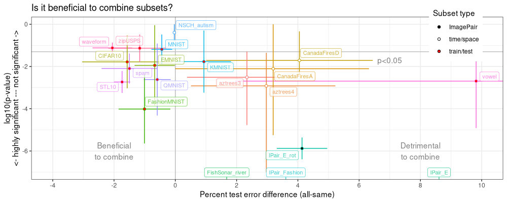
The SOAK figure above has one dot per data set, and segments which depict the range of P-values and test error differences, across the 2-4 data subsets. The values for each subset are in the table below:
(p.all <- p.each.group[compare_name=="all"])
##     subset_type            Data compare_name  test_subset      estimate      p.value compare_mean  same_mean
##          <char>          <char>       <fctr>       <char>         <num>        <num>        <num>      <num>
##  1:   ImagePair         IPair_E          all       EMNIST  9.052381e+00 6.527854e-12    15.479365  6.3771429
##  2:   ImagePair         IPair_E          all        MNIST  8.162724e+00 6.422049e-11    16.795679  8.6329553
##  3:   ImagePair     IPair_E_rot          all   EMNIST_rot  4.958730e+00 4.056908e-07    11.253968  6.3014286
##  4:   ImagePair     IPair_E_rot          all        MNIST  3.312752e+00 4.334588e-06    11.826428  8.5326816
##  5:   ImagePair   IPair_Fashion          all FashionMNIST  4.628571e+00 4.138273e-13    19.117143 14.4885714
##  6:   ImagePair   IPair_Fashion          all        MNIST  2.584307e+00 2.303932e-09    11.028558  8.4442508
##  7:  time/space    CanadaFiresA          all          306  6.321321e+00 8.250044e-03    10.180180  3.8588589
##  8:  time/space    CanadaFiresA          all          326  4.736858e-01 8.088654e-02     4.768774  4.2950879
##  9:  time/space    CanadaFiresA          all          329 -2.218278e-17 1.000000e+00     1.852726  1.8527264
## 10:  time/space    CanadaFiresA          all          395  5.978872e+00 5.671709e-06     8.794452  2.8155799
## 11:  time/space    CanadaFiresD          all          306  4.520617e+00 1.261188e-02     8.759807  4.2391899
## 12:  time/space    CanadaFiresD          all          326  4.222222e+00 5.639676e-03     9.777778  5.5555556
## 13:  time/space    CanadaFiresD          all          329  1.010753e+00 4.599875e-01     4.602151  3.5913978
## 14:  time/space    CanadaFiresD          all          395  6.444444e+00 4.331599e-03    10.444444  4.0000000
## 15:  time/space FishSonar_river          all          BOU  4.752551e-01 2.091857e-11    15.611503 15.1362481
## 16:  time/space FishSonar_river          all          CHI  1.289792e+00 2.093166e-12    30.094209 28.8044168
## 17:  time/space FishSonar_river          all          LEA  5.850666e-01 2.657473e-09    23.786981 23.2019142
## 18:  time/space FishSonar_river          all          PRL  4.364652e+00 4.317113e-15    30.749504 26.3848521
## 19:  time/space     NSCH_autism          all         2019 -6.589182e-02 1.614141e-01     2.527220  2.5931115
## 20:  time/space     NSCH_autism          all         2020 -1.163559e-05 9.997543e-01     2.405782  2.4057932
## 21:  time/space        aztrees3          all           NE  3.419998e+00 3.425018e-02     5.398379  1.9783804
## 22:  time/space        aztrees3          all           NW  3.833958e-01 5.063021e-02     1.213882  0.8304858
## 23:  time/space        aztrees3          all            S  3.208892e+00 1.692405e-05     3.379541  0.1706485
## 24:  time/space        aztrees4          all           NE  3.677197e+00 4.444655e-02     6.408536  2.7313391
## 25:  time/space        aztrees4          all           NW  5.124228e-01 3.669270e-02     1.342087  0.8296639
## 26:  time/space        aztrees4          all           SE  2.466950e+00 9.885714e-08     2.466950  0.0000000
## 27:  time/space        aztrees4          all           SW  5.224490e+00 1.318766e-02     5.224490  0.0000000
## 28:  train/test         CIFAR10          all         test -3.040000e+00 9.313619e-04    58.600000 61.6400000
## 29:  train/test         CIFAR10          all        train -1.020000e-01 2.934934e-01    58.746000 58.8480000
## 30:  train/test          EMNIST          all         test -1.330000e+00 1.422887e-04     6.420000  7.7500000
## 31:  train/test          EMNIST          all        train -1.666667e-02 9.071647e-01     6.410000  6.4759259
## 32:  train/test    FashionMNIST          all         test -1.850000e+00 2.279059e-06    15.490000 17.3400000
## 33:  train/test    FashionMNIST          all        train -1.616667e-01 4.126968e-03    14.273333 14.4350000
## 34:  train/test          KMNIST          all         test  1.820000e+00 5.767675e-04    28.050000 26.2300000
## 35:  train/test          KMNIST          all        train  4.666667e-02 5.030025e-01    17.846667 17.8000000
## 36:  train/test           MNIST          all         test -7.792532e-01 1.281417e-02     8.040451  8.8197042
## 37:  train/test           MNIST          all        train -1.033244e-01 3.280522e-01     8.606777  8.7101010
## 38:  train/test          QMNIST          all         test -1.500164e-01 1.224624e-01     7.521660  7.6716763
## 39:  train/test          QMNIST          all        train -1.028346e+00 4.766373e-05     7.599994  8.6283398
## 40:  train/test           STL10          all         test -1.475000e+00 5.647046e-04    61.875000 63.3500000
## 41:  train/test           STL10          all        train -2.000000e+00 6.068050e-03    62.920000 64.9200000
## 42:  train/test            spam          all         test -2.408148e+00 1.564139e-03     7.485434  9.8935821
## 43:  train/test            spam          all        train -5.868522e-01 4.129024e-02     7.799320  8.3861724
## 44:  train/test           vowel          all         test  1.768182e+01 1.213557e-05    34.409091 16.7272727
## 45:  train/test           vowel          all        train  1.954545e+00 3.428850e-01    32.045455 30.0909091
## 46:  train/test        waveform          all         test -1.408483e+00 4.226647e-02    15.177265 16.5857481
## 47:  train/test        waveform          all        train -2.701891e+00 1.362807e-01    17.315165 20.0170560
## 48:  train/test         zipUSPS          all         test -2.185365e+00 1.640868e-02     8.967641 11.1530060
## 49:  train/test         zipUSPS          all        train -1.384545e-01 3.293244e-01     5.045330  5.1837841
##     subset_type            Data compare_name  test_subset      estimate      p.value compare_mean  same_mean
##           log10.p    sign.log.p     N
##             <num>         <num> <int>
##  1: -1.118523e+01 11.1852295929    10
##  2: -1.019233e+01 10.1923263848    10
##  3: -6.391805e+00  6.3918048928    10
##  4: -5.363052e+00  5.3630521512    10
##  5: -1.238318e+01 12.3831808513    10
##  6: -8.637530e+00  8.6375303401    10
##  7: -2.083544e+00  2.0835437513    10
##  8: -1.092124e+00  1.0921237608    10
##  9:  0.000000e+00  0.0000000000    10
## 10: -5.246286e+00  5.2462860843    10
## 11: -1.899220e+00  1.8992202560    10
## 12: -2.248746e+00  2.2487458549    10
## 13: -3.372540e-01  0.3372539975    10
## 14: -2.363352e+00  2.3633517073    10
## 15: -1.067947e+01 10.6794680920    10
## 16: -1.167920e+01 11.6791963545    10
## 17: -8.575531e+00  8.5755311130    10
## 18: -1.436481e+01 14.3648065475    10
## 19: -7.920586e-01 -0.7920585547    10
## 20: -1.067407e-04 -0.0001067407    10
## 21: -1.465337e+00  1.4653371418    10
## 22: -1.295590e+00  1.2955902359    10
## 23: -4.771496e+00  4.7714958171    10
## 24: -1.352162e+00  1.3521619376    10
## 25: -1.435420e+00  1.4354203344    10
## 26: -7.004992e+00  7.0049919447    10
## 27: -1.879832e+00  1.8798322378    10
## 28: -3.030882e+00 -3.0308815501    10
## 29: -5.324016e-01 -0.5324016450    10
## 30: -3.846830e+00 -3.8468296945    10
## 31: -4.231388e-02 -0.0423138804    10
## 32: -5.642244e+00 -5.6422444862    10
## 33: -2.384369e+00 -2.3843689300    10
## 34: -3.238999e+00  3.2389991852    10
## 35: -2.984299e-01  0.2984298594    10
## 36: -1.892309e+00 -1.8923094823    10
## 37: -4.840571e-01 -0.4840570812    10
## 38: -9.119973e-01 -0.9119972530    10
## 39: -4.321812e+00 -4.3218119439    10
## 40: -3.248179e+00 -3.2481786513    10
## 41: -2.216951e+00 -2.2169508763    10
## 42: -2.805725e+00 -2.8057247785    10
## 43: -1.384153e+00 -1.3841526090    10
## 44: -4.915940e+00  4.9159398671    10
## 45: -4.648515e-01  0.4648515495    10
## 46: -1.374004e+00 -1.3740040048    10
## 47: -8.655658e-01 -0.8655657936    10
## 48: -1.784926e+00 -1.7849263105    10
## 49: -4.823761e-01 -0.4823760539    10
##           log10.p    sign.log.p     N
The table above has one row per subset in each of the data sets. To make a volcano plot, we need to invert the Y axis, and remove the segments.
text.y <- -6.5
text.dt <- rbind(
  tlab(7, -1.4, "p<0.05"),
  tlab(-2, text.y, "Beneficial\nto combine"),
  tlab(8, text.y, "Detrimental\nto combine"))
ggplot()+
  theme_bw()+
  theme(legend.position=c(0.9,0.1))+
  geom_hline(yintercept=-log10(0.05),color="grey")+
  geom_vline(xintercept=0,color="grey")+
  geom_text(aes(
    x, -y, label=label, color=NULL),
    color="grey50",
    data=text.dt)+
  geom_point(aes(
    estimate, -log10.p,
    color=Data,
    fill=subset_type),
    shape=21,
    data=p.all)+
  ggrepel::geom_label_repel(aes(
    estimate, -log10.p, color=Data,
    label=sprintf("%s\n%s",Data,test_subset)),
    alpha=0.75,
    size=2.8,
    data=p.all)+
  scale_fill_manual(
    "Subset type", values=type.colors)+
  scale_color_discrete(guide="none")+
  scale_y_continuous(
    "-log10(p-value)\n<- not significant --- highly significant ->",
    breaks=seq(-100,100,by=2))+
  scale_x_continuous(
    "Percent test error difference (all-same)",
    breaks=seq(-100,10,by=2))+
  coord_cartesian(
    xlim=c(-4,10),
    ylim=c(0,7))
## Warning: ggrepel: 3 unlabeled data points (too many overlaps). Consider increasing max.overlaps
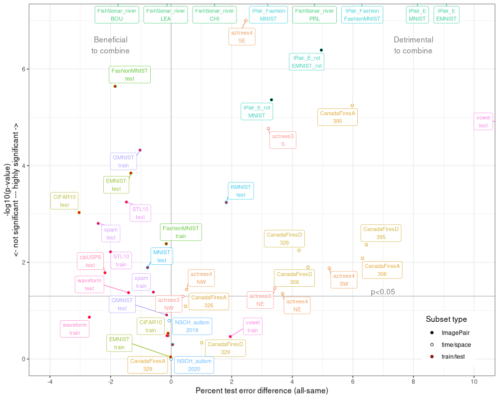
The result above has one dot (and label) for each data subset. The dots appear to have a distribution which is somewhat similar to the characteristic V pattern in volcano plots.
Conclusions
We have shown how to make volcano plots using SOAK subset data.
Session Info
sessionInfo()
## R version 4.5.0 (2025-04-11)
## Platform: x86_64-pc-linux-gnu
## Running under: Ubuntu 24.04.2 LTS
##
## Matrix products: default
## BLAS:   /usr/lib/x86_64-linux-gnu/blas/libblas.so.3.12.0
## LAPACK: /usr/lib/x86_64-linux-gnu/lapack/liblapack.so.3.12.0  LAPACK version 3.12.0
##
## locale:
##  [1] LC_CTYPE=fr_FR.UTF-8       LC_NUMERIC=C               LC_TIME=fr_FR.UTF-8        LC_COLLATE=fr_FR.UTF-8
##  [5] LC_MONETARY=fr_FR.UTF-8    LC_MESSAGES=fr_FR.UTF-8    LC_PAPER=fr_FR.UTF-8       LC_NAME=C
##  [9] LC_ADDRESS=C               LC_TELEPHONE=C             LC_MEASUREMENT=fr_FR.UTF-8 LC_IDENTIFICATION=C
##
## time zone: Europe/Paris
## tzcode source: system (glibc)
##
## attached base packages:
## [1] stats     graphics  grDevices utils     datasets  methods   base
##
## other attached packages:
## [1] ggplot2_3.5.1     data.table_1.17.0
##
## loaded via a namespace (and not attached):
##  [1] directlabels_2024.1.21 crayon_1.5.3           vctrs_0.6.5            cli_3.6.4              knitr_1.50
##  [6] xfun_0.51              rlang_1.1.5            ggrepel_0.9.6          bench_1.1.4            generics_0.1.3
## [11] glue_1.8.0             labeling_0.4.3         nc_2025.3.24           colorspace_2.1-1       scales_1.3.0
## [16] fpopw_1.1              quadprog_1.5-8         grid_4.5.0             evaluate_1.0.3         munsell_0.5.1
## [21] tibble_3.2.1           profmem_0.6.0          lifecycle_1.0.4        compiler_4.5.0         dplyr_1.1.4
## [26] Rcpp_1.0.14            pkgconfig_2.0.3        atime_2025.4.1         farver_2.1.2           lattice_0.22-6
## [31] R6_2.6.1               tidyselect_1.2.1       pillar_1.10.1          magrittr_2.0.3         tools_4.5.0
## [36] withr_3.0.2            gtable_0.3.6