Centralized vs de-centralized parallelization
I recently wrote about New parallel computing frameworks in R, including the rush package by Marc Becker, who I met in a visit to Bernd Bischl’s lab in Munich this week. One of the main ideas of rush is de-centralized parallelism, meaning there is no central server that assigns tasks to workers. Instead, each worker decides what task to work on, which can be much faster in some applications. The goal of this blog was to explore one such application where these different methods of parallel computation can be applied: optimal change-point detection algorithms.
Introduction to peak detection in genomic data
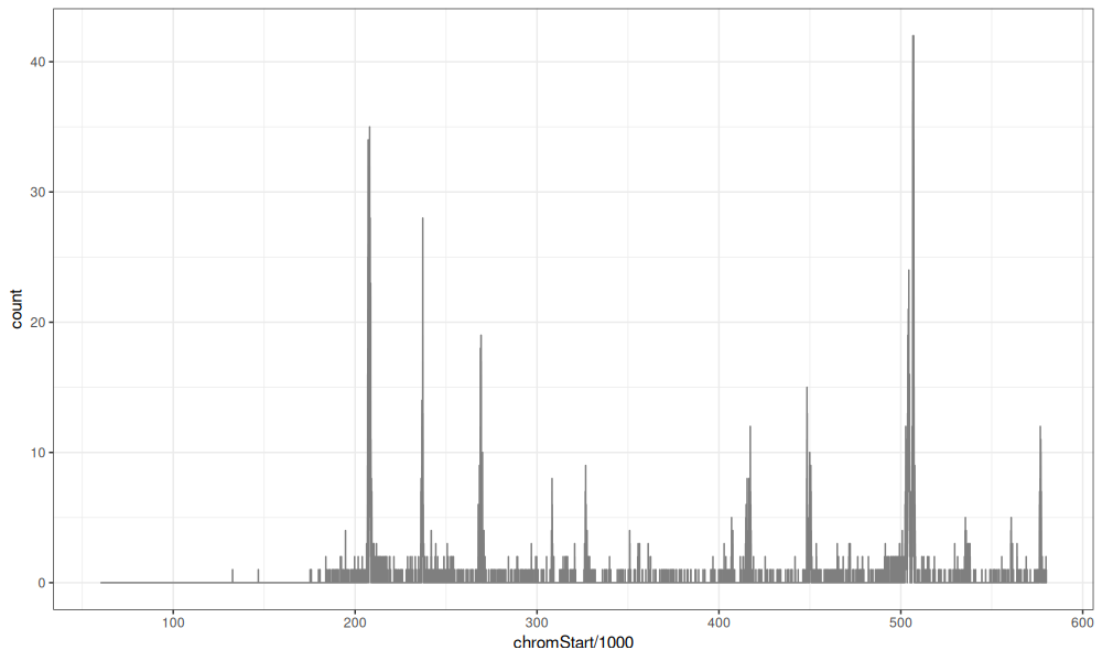
In the PeakSegDisk package, we have the Mono27ac data set, which
represents part of a genomic profile, with several peaks that
represent active regions.
data(Mono27ac, package="PeakSegDisk")
library(data.table)
Mono27ac$coverage
##        chrom chromStart chromEnd count
##       <char>      <int>    <int> <int>
##    1:  chr11      60000   132601     0
##    2:  chr11     132601   132643     1
##    3:  chr11     132643   146765     0
##    4:  chr11     146765   146807     1
##    5:  chr11     146807   175254     0
##   ---
## 6917:  chr11     579752   579792     1
## 6918:  chr11     579792   579794     2
## 6919:  chr11     579794   579834     1
## 6920:  chr11     579834   579980     0
## 6921:  chr11     579980   580000     1
These data can be visualized via the code below.
library(ggplot2)
ggplot()+
  theme_bw()+
  geom_step(aes(
    chromStart/1e3, count),
    color="grey50",
    data=Mono27ac$coverage)
Computing a peak model
We may like to compute a sequence of change-point models for these
data. In the PeakSegDisk package, you can use the
sequentialSearch_dir function to compute a model with a given number
of peaks. You first must save the data to disk, as in the code below.
data.dir <- file.path(
  tempfile(),
  "H3K27ac-H3K4me3_TDHAM_BP",
  "samples",
  "Mono1_H3K27ac",
  "S001YW_NCMLS",
  "problems",
  "chr11-60000-580000")
dir.create(data.dir, recursive=TRUE, showWarnings=FALSE)
write.table(
  Mono27ac$coverage, file.path(data.dir, "coverage.bedGraph"),
  col.names=FALSE, row.names=FALSE, quote=FALSE, sep="\t")
After that, you can run the sequential search algorithm, in parallel if you declare a future plan as in the code below.
future::plan("multisession")
fit10 <- PeakSegDisk::sequentialSearch_dir(data.dir, 10L, verbose=1)
## Next = 0, Inf
## Next = 157.994737329317
## Next = 1952.66876946418
## Next = 21915.161494366
## Next = 6699.96265606243
## Next = 3738.08792382758
## Next = 5674.91008099583
The code uses a penalized solver, which means a non-negative penalty value must be specified as the model complexity hyper-parameter, and we do not know in advance how many change-points (and peaks) that will give. The sequential search algorithm evaluates a bunch of different penalty values until it finds the desired number of peaks (10 in this case). This model is shown below,
plot(fit10)+
  geom_step(aes(
    chromStart, count),
    color="grey50",
    data=Mono27ac$coverage)
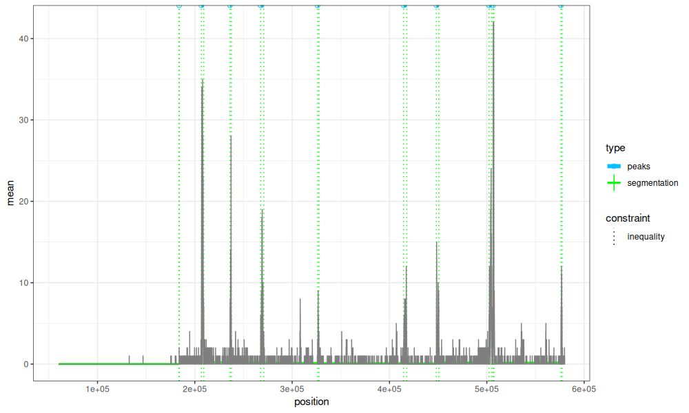
The plot above shows that the model change-points are a reasonable fit to the data, but we may want to examine other model sizes (say from 5 to 15 peaks).
target.min.peaks <- 5
target.max.peaks <- 15
To do that, we could implement a parallel computation of
the penalty values. Next output above shows the penalties that were
evaluated in the search. We see that the first two penalties are 0
and Inf, which give the largest/smallest change-point models (3199
and 0 peaks in this case). Those are the only two that are evaluated
in parallel. Next, we show how we could evaluate several penalties in
parallel.
Computing a range of models
Computing a range of change-point model sizes can be implemented using the CROCS algorithm, described in our BMC Bioinformatics 2021 paper, with Arnaud Liehrmann and Guillem Rigaill. To do that, we first compute the most extreme models.
pen.vec <- c(0,Inf)
loss.dt.list <- list()
for(pen in pen.vec){
  fit <- PeakSegDisk::PeakSegFPOP_dir(data.dir, pen)
  loss.dt.list[[paste(pen)]] <- fit$loss[, .(penalty, peaks, total.loss)]
}
(loss.dt <- rbindlist(loss.dt.list))
##    penalty peaks total.loss
##      <num> <int>      <num>
## 1:       0  3199  -130227.3
## 2:     Inf     0   375197.9
The table above shows the number of peaks and Poisson loss values for the two models. The optimization objective is the cost plus the penalty times the number of peaks. Therefore, the number of peaks selected for a given penalty is the argmin of a finite number of linear functions. Each linear function has slope equal to number of peaks, and intercept equal to total Poisson loss. We can compute an estimate of a model selection function, which maps penalty/lambda values to model sizes (in peaks) via the code below.
get_selection <- function(loss){
  selection.df <- penaltyLearning::modelSelection(loss, "total.loss", "peaks")
  with(selection.df, data.table(
    total.loss,
    min.lambda,
    penalty,
    max.lambda,
    peaks_after=c(peaks[-1],NA),
    peaks
  ))[
  , helpful := peaks_after<target.max.peaks & peaks>target.min.peaks &
      peaks_after+1 < peaks & !max.lambda %in% names(loss.dt.list)
  ][]
}
(selection.dt <- get_selection(loss.dt))
##    total.loss min.lambda penalty max.lambda peaks_after peaks helpful
##         <num>      <num>   <num>      <num>       <int> <int>  <lgcl>
## 1:  -130227.3     0.0000       0   157.9947           0  3199    TRUE
## 2:   375197.9   157.9947     Inf        Inf          NA     0   FALSE
The table above has columns for min.lambda and max.lambda, which
indicate a range of penalties for which we have evidence that peaks
may be selected. We can visualize these functions via the plot below,
get_gg <- function(){
  dot.dt <- rbind(
    data.table(loss.dt[, .(
      penalty, peaks, total.loss, helpful=FALSE)], dot="evaluated"),
    data.table(selection.dt[-.N, .(
      penalty=max.lambda, peaks, total.loss, helpful)], dot="candidate"))
  ggplot()+
    geom_abline(aes(
      slope=peaks,
      intercept=total.loss),
      data=loss.dt)+
    geom_point(aes(
      penalty,
      total.loss+ifelse(peaks==0, 0, penalty*peaks),
      color=helpful),
      size=5,
      data=dot.dt)+
    geom_point(aes(
      penalty,
      total.loss+ifelse(peaks==0, 0, penalty*peaks),
      color=helpful,
      fill=dot),
      shape=21,
      size=4,
      data=dot.dt)+
    geom_label(aes(
      penalty,
      total.loss+ifelse(peaks==0, 0, penalty*peaks),
      hjust=ifelse(penalty==Inf, 1, 0.5),
      label=peaks),
      vjust=1.5,
      alpha=0.5,
      data=dot.dt[dot=="evaluated"])+
    scale_fill_manual(values=c(evaluated="white", candidate="black"))+
    scale_color_manual(values=c("TRUE"="red", "FALSE"="black"))+
    scale_y_continuous("Cost = Loss + penalty * peaks")
}
get_gg()
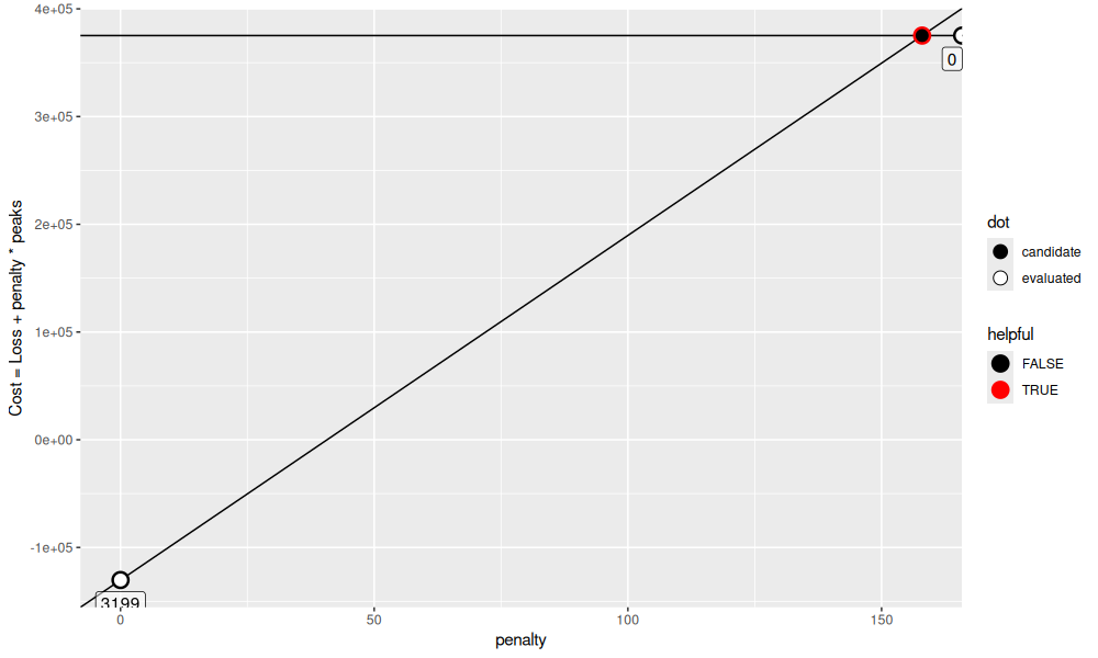
pen <- selection.dt$max.lambda[1]
We see in the plot above that there is an intersection of these functions at penalty=157.9947373. Since these functions are for 3199 and 0 peaks, and our target numbers of peaks is between (5 to 15), we are guaranteed to make progress if we compute a new penalty at the intersection point. We do that in the code below,
fit <- PeakSegDisk::PeakSegFPOP_dir(data.dir, pen)
loss.dt.list[[paste(pen)]] <- fit$loss[, .(penalty, peaks, total.loss)]
(loss.dt <- rbindlist(loss.dt.list))
##     penalty peaks total.loss
##       <num> <int>      <num>
## 1:   0.0000  3199 -130227.29
## 2:      Inf     0  375197.87
## 3: 157.9947   224  -62199.93
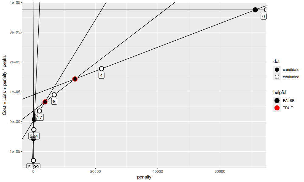
We see in the new loss table that there is an intermediate number of peaks, 224. This results in two intersection point candidates (the first two rows of the table below).
(selection.dt <- get_selection(loss.dt))
##    total.loss min.lambda  penalty max.lambda peaks_after peaks helpful
##         <num>      <num>    <num>      <num>       <int> <int>  <lgcl>
## 1: -130227.29    0.00000   0.0000   22.86634         224  3199   FALSE
## 2:  -62199.93   22.86634 157.9947 1952.66877           0   224    TRUE
## 3:  375197.87 1952.66877      Inf        Inf          NA     0   FALSE
get_gg()
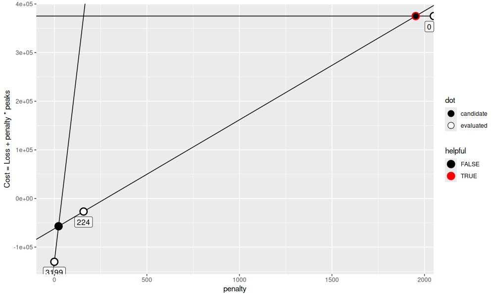
We see in the figure above that only one of the two candidates is helpful toward our goal of computing models between 5 and 15 peaks. We can evaluate the penalty at that candidate in order to make progress. Let’s keep going until we have more than one interesting/helpful candidate.
while(sum(selection.dt$helpful)==1){
  pen <- selection.dt[helpful==TRUE, max.lambda]
  fit <- PeakSegDisk::PeakSegFPOP_dir(data.dir, pen)
  print(loss.dt.list[[paste(pen)]] <- fit$loss[, .(penalty, peaks, total.loss)])
  loss.dt <- rbindlist(loss.dt.list)
  selection.dt <- get_selection(loss.dt)
}
##     penalty peaks total.loss
##       <num> <int>      <num>
## 1: 1952.669    17   2640.128
##     penalty peaks total.loss
##       <num> <int>      <num>
## 1: 21915.16     4   89739.64
##     penalty peaks total.loss
##       <num> <int>      <num>
## 1: 6699.963     8   36282.92
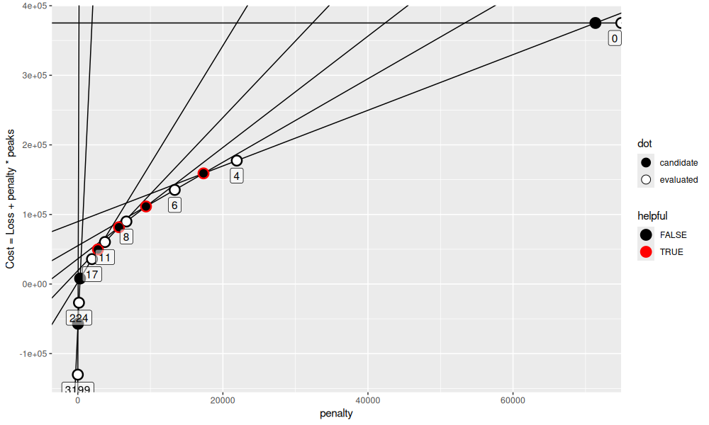
selection.dt
##     total.loss  min.lambda    penalty  max.lambda peaks_after peaks helpful
##          <num>       <num>      <num>       <num>       <int> <int>  <lgcl>
## 1: -130227.291     0.00000     0.0000    22.86634         224  3199   FALSE
## 2:  -62199.931    22.86634   157.9947   313.23700          17   224   FALSE
## 3:    2640.128   313.23700  1952.6688  3738.08792           8    17    TRUE
## 4:   36282.919  3738.08792  6699.9627 13364.18080           4     8    TRUE
## 5:   89739.642 13364.18080 21915.1615 71364.55772           0     4   FALSE
## 6:  375197.873 71364.55772        Inf         Inf          NA     0   FALSE
The output above shows that there are now two helpful candidates. The code below visualizes them.
get_gg()
Above we see that there are 5 candidate penalties, but only 2 helpful penalties that would make progress toward computing all models between 5 and 15 peaks. At this point we may think of how to parallelize.
Centralized launching
One way to parallelize the computation is by first computing the candidate penalties in a central process, then sending those penalties to workers for computation.
Centralized parallelization via future.apply
We use future.apply to implement the central launcher method in the code below.
pen.list <- list()
seq_it <- function(){
pen.vec <- selection.dt[helpful==TRUE, max.lambda]
pen.list[[length(pen.list)+1]] <<- pen.vec
loss.dt.list[paste(pen.vec)] <<- future.apply::future_lapply(pen.vec, function(pen){
fit <- PeakSegDisk::PeakSegFPOP_dir(data.dir, pen)
fit$loss[, .(penalty, peaks, total.loss)]
})
loss.dt <<- rbindlist(loss.dt.list)
selection.dt <<- get_selection(loss.dt)
get_gg()
}
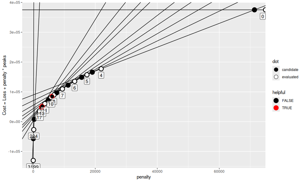
seq_it()
After the first parallel iteration above, we see four helpful candidates.
seq_it()
Let’s keep going.
while(any(selection.dt$helpful)){
  gg <- seq_it()
}
gg
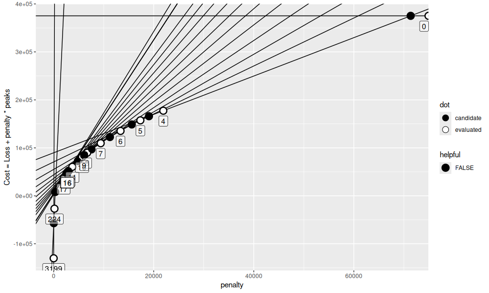
selection.dt
##      total.loss  min.lambda    penalty  max.lambda peaks_after peaks helpful
##           <num>       <num>      <num>       <num>       <int> <int>  <lgcl>
##  1: -130227.291     0.00000     0.0000    22.86634         224  3199   FALSE
##  2:  -62199.931    22.86634   157.9947   313.23700          17   224   FALSE
##  3:    2640.128   313.23700  1952.6688  2512.24686          16    17   FALSE
##  4:    5152.375  2512.24686  2729.6793  2729.67926          14    16   FALSE
##  5:   10611.733  2729.67926  2740.3022  2761.54815          13    14   FALSE
##  6:   13373.281  2761.54815  2769.6768  2868.53480          12    13   FALSE
##  7:   16241.816  2868.53480  2942.4538  3016.37275          11    12   FALSE
##  8:   19258.189  3016.37275  3738.0879  4850.20081          10    11   FALSE
##  9:   24108.390  4850.20081  5674.9101  5956.50214           9    10   FALSE
## 10:   30064.892  5956.50214  6087.2647  6218.02730           8     9   FALSE
## 11:   36282.919  6218.02730  6699.9627  7562.33626           7     8   FALSE
## 12:   43845.255  7562.33626  9400.8673 11239.39840           6     7   FALSE
## 13:   55084.654 11239.39840 13364.1808 15609.51789           5     6   FALSE
## 14:   70694.172 15609.51789 17327.4943 19045.47066           4     5   FALSE
## 15:   89739.642 19045.47066 21915.1615 71364.55772           0     4   FALSE
## 16:  375197.873 71364.55772        Inf         Inf          NA     0   FALSE
We see in the table above that there are 16 iterations total.
Coding a cenral launcher function
Overall the algorithm which uses a central launcher to determine candidates can be implemented via the code below.
central_launch <- function(target.min.peaks, target.max.peaks, LAPPLY=future.apply::future_lapply){
  data.dir <- file.path(
    tempfile(),
    "H3K27ac-H3K4me3_TDHAM_BP",
    "samples",
    "Mono1_H3K27ac",
    "S001YW_NCMLS",
    "problems",
    "chr11-60000-580000")
  dir.create(data.dir, recursive=TRUE, showWarnings=FALSE)
  write.table(
    Mono27ac$coverage, file.path(data.dir, "coverage.bedGraph"),
    col.names=FALSE, row.names=FALSE, quote=FALSE, sep="\t")
  pen.vec <- c(0,Inf)
  loss.dt.list <- list()
  cand.dt.list <- list()
  iteration <- 1L
  while(length(pen.vec)){
    loss.dt.list[paste(pen.vec)] <- LAPPLY(
      pen.vec, function(pen){
        start.time <- Sys.time()
        fit <- PeakSegDisk::PeakSegFPOP_dir(data.dir, pen)
        fit$loss[, .(
          penalty, peaks, total.loss, iteration,
          process=factor(Sys.getpid()), start.time, end.time=Sys.time())]
      }
    )
    start.time <- Sys.time()
    loss.dt <- rbindlist(loss.dt.list)
    selection.df <- penaltyLearning::modelSelection(loss.dt, "total.loss", "peaks")
    selection.dt <- with(selection.df, data.table(
      total.loss,
      min.lambda,
      penalty,
      max.lambda,
      peaks_after=c(peaks[-1],NA),
      peaks
    ))[
    , helpful := peaks_after<target.max.peaks & peaks>target.min.peaks &
        peaks_after+1 < peaks & !max.lambda %in% names(loss.dt.list)
    ][]
    pen.vec <- selection.dt[helpful==TRUE, max.lambda]
    cand.dt.list[[length(cand.dt.list)+1]] <- data.table(
      iteration,
      process=factor(Sys.getpid()), start.time, end.time=Sys.time())
    iteration <- iteration+1L
  }
  list(loss=loss.dt, candidates=rbindlist(cand.dt.list))
}
(loss_5_15 <- central_launch(5,15))
## $loss
##        penalty peaks  total.loss iteration process          start.time            end.time
##          <num> <int>       <num>     <int>  <fctr>              <POSc>              <POSc>
##  1:     0.0000  3199 -130227.291         1 1782423 2025-07-04 12:43:46 2025-07-04 12:43:46
##  2:        Inf     0  375197.873         1 1782422 2025-07-04 12:43:46 2025-07-04 12:43:46
##  3:   157.9947   224  -62199.931         2 1782423 2025-07-04 12:43:47 2025-07-04 12:43:47
##  4:  1952.6688    17    2640.128         3 1782423 2025-07-04 12:43:48 2025-07-04 12:43:48
##  5: 21915.1615     4   89739.642         4 1782423 2025-07-04 12:43:49 2025-07-04 12:43:49
##  6:  6699.9627     8   36282.919         5 1782423 2025-07-04 12:43:50 2025-07-04 12:43:50
##  7:  3738.0879    11   19258.189         6 1782423 2025-07-04 12:43:50 2025-07-04 12:43:51
##  8: 13364.1808     6   55084.654         6 1782422 2025-07-04 12:43:51 2025-07-04 12:43:51
##  9:  2769.6768    13   13373.281         7 1782423 2025-07-04 12:43:51 2025-07-04 12:43:52
## 10:  5674.9101    10   24108.390         7 1782422 2025-07-04 12:43:52 2025-07-04 12:43:52
## 11:  9400.8673     7   43845.255         7 1782424 2025-07-04 12:43:52 2025-07-04 12:43:52
## 12: 17327.4943     5   70694.172         7 1782420 2025-07-04 12:43:52 2025-07-04 12:43:53
## 13:  2683.2884    16    5152.375         8 1782423 2025-07-04 12:43:53 2025-07-04 12:43:54
## 14:  2942.4538    12   16241.816         8 1782422 2025-07-04 12:43:54 2025-07-04 12:43:54
## 15:  6087.2647     9   30064.892         8 1782424 2025-07-04 12:43:54 2025-07-04 12:43:54
## 16:  2740.3022    14   10611.733         9 1782423 2025-07-04 12:43:54 2025-07-04 12:43:55
## 17:  2729.6793    16    5152.375        10 1782423 2025-07-04 12:43:55 2025-07-04 12:43:56
## 18:  2729.6793    16    5152.375        11 1782423 2025-07-04 12:43:56 2025-07-04 12:43:57
##
## $candidates
##     iteration process          start.time            end.time
##         <int>  <fctr>              <POSc>              <POSc>
##  1:         1 1782323 2025-07-04 12:43:46 2025-07-04 12:43:46
##  2:         2 1782323 2025-07-04 12:43:47 2025-07-04 12:43:47
##  3:         3 1782323 2025-07-04 12:43:48 2025-07-04 12:43:48
##  4:         4 1782323 2025-07-04 12:43:49 2025-07-04 12:43:49
##  5:         5 1782323 2025-07-04 12:43:50 2025-07-04 12:43:50
##  6:         6 1782323 2025-07-04 12:43:51 2025-07-04 12:43:51
##  7:         7 1782323 2025-07-04 12:43:53 2025-07-04 12:43:53
##  8:         8 1782323 2025-07-04 12:43:54 2025-07-04 12:43:54
##  9:         9 1782323 2025-07-04 12:43:55 2025-07-04 12:43:55
## 10:        10 1782323 2025-07-04 12:43:56 2025-07-04 12:43:56
## 11:        11 1782323 2025-07-04 12:43:57 2025-07-04 12:43:57
The result is a list of two tables:
losshas one row per penalty value computed.candidateshas one row per computation of new candidates.
To visualize these results, I coded a special Positioning Method for directlabels::geom_dl below.
viz_workers <- function(L){
  min.time <- min(L$loss$start.time)
  for(N in names(L)){
    L[[N]] <- data.table(L[[N]], computation=N)
    for(pos in c("start", "end")){
      time.vec <- L[[N]][[paste0(pos,".time")]]
      set(L[[N]], j=paste0(pos,".seconds"), value=time.vec-min.time)
    }
  }
  ##L$cand$process <- L$loss[, .(count=.N), by=process][order(-count)][1, process]
  biggest.diff <- L$loss[,as.numeric(diff(c(min(start.seconds),max(end.seconds))))]
  n.proc <- length(unique(L$loss$process))
  best.seconds <- n.proc*biggest.diff
  total.seconds <- L$loss[,sum(end.seconds-start.seconds)]
  efficiency <- total.seconds/best.seconds
  seg.dt <- rbind(L$cand,L$loss[,names(L$cand),with=FALSE])
  proc.levs <- unique(c(levels(L$cand$process), levels(L$loss$process)))
  text.dt <- L$loss[,.(
    mid.seconds=as.POSIXct((as.numeric(min(start.seconds))+as.numeric(max(end.seconds)))/2),
    label=paste(peaks,collapse=",")
  ),by=.(process,iteration)]
  it.dt <- seg.dt[, .(min.seconds=min(start.seconds), max.seconds=max(end.seconds)), by=iteration]
  comp.colors <- c(
    loss="black",
    candidates="red")
  ggplot()+
    theme_bw()+
    ggtitle(sprintf("Worker efficiency = %.1f%%", 100*total.seconds/best.seconds))+
    geom_rect(aes(
      xmin=min.seconds, xmax=max.seconds,
      ymin=-Inf, ymax=Inf),
      fill="grey",
      color="white",
      alpha=0.5,
      data=it.dt)+
    geom_text(aes(
      x=(min.seconds+max.seconds)/2, Inf,
      hjust=ifelse(iteration==1, 1, 0.5),
      label=paste0(ifelse(iteration==1, "it=", ""), iteration)),
      data=it.dt,
      vjust=1)+
    directlabels::geom_dl(aes(
      start.seconds, process,
      label.group=paste(iteration, process),
      label=peaks),
      data=L$loss,
      method=polygon.mine("bottom", offset.cm=0.2, custom.colors=list(box.color="white")))+
    geom_segment(aes(
      start.seconds, process,
      color=computation,
      xend=end.seconds, yend=process),
      data=seg.dt)+
    geom_point(aes(
      start.seconds, process,
      color=computation),
      shape=1,
      data=seg.dt)+
    scale_color_manual(
      values=comp.colors,
      limits=names(comp.colors))+
    scale_y_discrete(
      limits=proc.levs, # necessary for red dot on bottom.
      name="process")+
    scale_x_continuous("time (seconds)")
}
polygon.mine <- function
### Make a Positioning Method that places non-overlapping speech
### polygons at the first or last points.
(top.bottom.left.right,
### Character string indicating what side of the plot to label.
  offset.cm=0.1,
### Offset from the polygon to the most extreme data point.
  padding.cm=0.05,
### Padding inside the polygon.
  custom.colors=NULL
### Positioning method applied just before draw.polygons, can set
### box.color and text.color for custom colors.
){
  if(is.null(custom.colors)){
    custom.colors <- directlabels::gapply.fun({
      rgb.mat <- col2rgb(d[["colour"]])
      d$text.color <- with(data.frame(t(rgb.mat)), {
        gray <- 0.3*red + 0.59*green + 0.11*blue
        ifelse(gray/255 < 0.5, "white", "black")
      })
      d
    })
  }
  opposite.side <- c(
    left="right",
    right="left",
    top="bottom",
    bottom="top")[[top.bottom.left.right]]
  direction <- if(
    top.bottom.left.right %in% c("bottom", "left")
  ) -1 else 1
  min.or.max <- if(
    top.bottom.left.right %in% c("top", "right")
  ) max else min
  if(top.bottom.left.right %in% c("left", "right")){
    min.or.max.xy <- "x"
    qp.target <- "y"
    qp.max <- "top"
    qp.min <- "bottom"
    padding.h.factor <- 2
    padding.w.factor <- 1
    limits.fun <- ylimits
    reduce.method <- "reduce.cex.lr"
  }else{
    min.or.max.xy <- "y"
    qp.target <- "x"
    qp.max <- "right"
    qp.min <- "left"
    padding.h.factor <- 1
    padding.w.factor <- 2
    limits.fun <- directlabels::xlimits
    reduce.method <- "reduce.cex.tb"
  }
  list(
    hjust=0.5, vjust=1,
    function(d,...){
      ## set the end of the speech polygon to the original data point.
      for(xy in c("x", "y")){
        extra.coord <- sprintf(# e.g. left.x
          "%s.%s", opposite.side, xy)
        d[[extra.coord]] <- d[[xy]]
      }
      ## offset positions but do NOT set the speech polygon position
      ## to the min or max.
      d[[min.or.max.xy]] <- d[[min.or.max.xy]] + offset.cm*direction
      d
    },
    "calc.boxes",
    reduce.method,
    function(d, ...){
      d$h <- d$h + padding.cm * padding.h.factor
      d$w <- d$w + padding.cm * padding.w.factor
      d
    },
    "calc.borders",
    function(d,...){
      do.call(rbind, lapply(split(d, d$y), function(d){
        directlabels::apply.method(directlabels::qp.labels(
          qp.target,
          qp.min,
          qp.max,
          directlabels::make.tiebreaker(min.or.max.xy, qp.target),
          limits.fun), d)
      }))
    },
    "calc.borders",
    custom.colors,
    "draw.polygons")
}
viz_workers(loss_5_15)
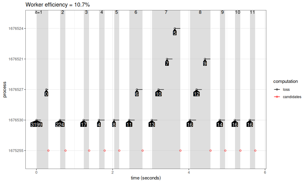
The figure above shows how the computation proceeds over time (X axis) in the different parallel processes (Y axis). Iterations are shown in grey rectangles, with iteration numbers at the top of the plot. In each iteration, There are at most four parallel workers (black) at any given time. We see that before starting a new iteration, all workers must complete, and wait for the central process to compute new candidates. The worker efficiency reported at the top of the plot is the amount of time taken computing models (black segments), divided by the max time that could be taken by that number of workers (if black line segments were from start to end of the plot for each worker). There are two sources of inefficiency:
- The overhead for starting a new future job is about 0.2 seconds, and this overhead could be reduced by using mirai package instead. But for long running computations (big data or complex models), this overhead is not the important bottleneck.
- Because of the centralized method for computing new candidates, the first process that finishes in an iteration must wait for the last process, before it starts working again. This can be fixed by using rush package instead (as we show in the next section).
To see these patterns more clearly, below we run the central launch algorithm with a larger number of models:
results_1_100 <- list()
(results_1_100$future_lapply <- central_launch(1,100))
## $loss
##        penalty peaks  total.loss iteration process          start.time            end.time
##          <num> <int>       <num>     <int>  <fctr>              <POSc>              <POSc>
##   1:    0.0000  3199 -130227.291         1 1782423 2025-07-04 12:43:58 2025-07-04 12:43:58
##   2:       Inf     0  375197.873         1 1782422 2025-07-04 12:43:58 2025-07-04 12:43:58
##   3:  157.9947   224  -62199.931         2 1782423 2025-07-04 12:43:59 2025-07-04 12:43:59
##   4: 1952.6688    17    2640.128         3 1782423 2025-07-04 12:44:00 2025-07-04 12:44:00
##   5:  313.2370    74  -31865.715         4 1782423 2025-07-04 12:44:00 2025-07-04 12:44:01
##  ---
## 112:  314.0074    74  -31865.715        13 1782420 2025-07-04 12:44:40 2025-07-04 12:44:40
## 113:  327.0344    62  -28011.480        13 1782425 2025-07-04 12:44:40 2025-07-04 12:44:40
## 114:  247.0699    95  -37499.236        14 1782423 2025-07-04 12:44:41 2025-07-04 12:44:41
## 115:  247.5600    95  -37499.236        14 1782422 2025-07-04 12:44:41 2025-07-04 12:44:41
## 116:  327.0344    62  -28011.480        14 1782424 2025-07-04 12:44:42 2025-07-04 12:44:42
##
## $candidates
##     iteration process          start.time            end.time
##         <int>  <fctr>              <POSc>              <POSc>
##  1:         1 1782323 2025-07-04 12:43:58 2025-07-04 12:43:58
##  2:         2 1782323 2025-07-04 12:43:59 2025-07-04 12:43:59
##  3:         3 1782323 2025-07-04 12:44:00 2025-07-04 12:44:00
##  4:         4 1782323 2025-07-04 12:44:01 2025-07-04 12:44:01
##  5:         5 1782323 2025-07-04 12:44:02 2025-07-04 12:44:02
##  6:         6 1782323 2025-07-04 12:44:06 2025-07-04 12:44:06
##  7:         7 1782323 2025-07-04 12:44:09 2025-07-04 12:44:09
##  8:         8 1782323 2025-07-04 12:44:15 2025-07-04 12:44:15
##  9:         9 1782323 2025-07-04 12:44:20 2025-07-04 12:44:20
## 10:        10 1782323 2025-07-04 12:44:27 2025-07-04 12:44:27
## 11:        11 1782323 2025-07-04 12:44:34 2025-07-04 12:44:34
## 12:        12 1782323 2025-07-04 12:44:38 2025-07-04 12:44:38
## 13:        13 1782323 2025-07-04 12:44:40 2025-07-04 12:44:40
## 14:        14 1782323 2025-07-04 12:44:42 2025-07-04 12:44:42
viz_workers(results_1_100$future_lapply)
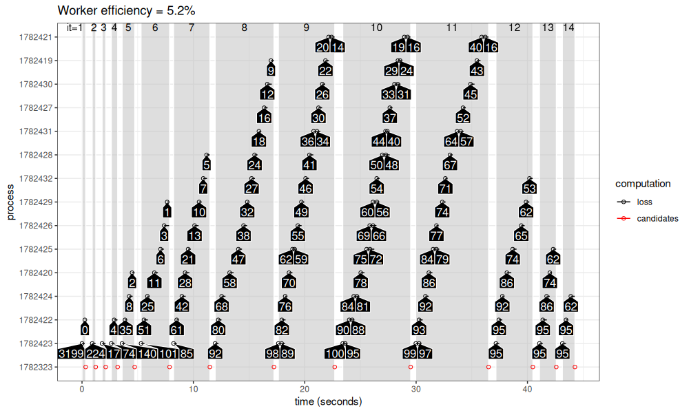
The figure above shows more iterations and more processes. In some iterations (9-11), the number of candidates is greater than 14, which is the number of CPUs on my machine (and the max number of future workers). In those iterations, we see calculation of either 1 or 2 models in each worker process.
Centralized launching, no parallelization
A baseline to compare is no parallel computation (everything in one process), as coded below.
results_1_100$lapply <- central_launch(1,100,lapply)
viz_workers(results_1_100$lapply)
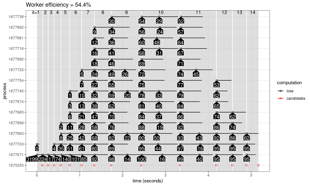
The result above is almost 100% efficient (because only one CPU is used instead of 14), but it takes longer overall.
Centralized launching, mirai
Another comparison is mirai, which offers lower overhead than future.
if(mirai::daemons()$connections==0){
mirai::daemons(future::availableCores())
}
results_1_100$mirai_map <- central_launch(1,100,function(...){
mirai::mirai_map(...)[]
})
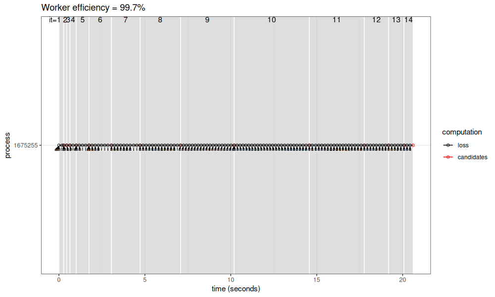
viz_workers(results_1_100$mirai_map)
The figure above shows that there is very little overhead for launching mirai parallel tasks. In each iteration, we can see that all 14 processes start almost at the same time. This results in a shorter overall comptutation time. However, we can see still some overhead/inefficiency that comes from the centralized computation of target penalties. That is, at each iteration, some processes are short, and must wait until the longest process in the iteration finishes, before receiving a new penalty to compute. This observation motivates the de-centralized parallelized model that should be possible using rush.
Comparison of central launching methods
In the code below, we combine the results from the three methods in the previous sections.
loss_1_100_list <- list()
fun_levs <- c("lapply", "future_lapply", "mirai_map")
for(fun in names(results_1_100)){
  loss_fun <- results_1_100[[fun]]$loss
  min.time <- min(loss_fun$start.time)
  loss_1_100_list[[fun]] <- data.table(fun=factor(fun, fun_levs), loss_fun)[, let(
    process_i = as.integer(process),
    start.time=start.time-min.time,
    end.time=end.time-min.time)]
}
(loss_1_100 <- rbindlist(loss_1_100_list))
##                fun   penalty peaks  total.loss iteration process     start.time       end.time process_i
##             <fctr>     <num> <int>       <num>     <int>  <fctr>     <difftime>     <difftime>     <int>
##   1: future_lapply    0.0000  3199 -130227.291         1 1782423 0.0000000 secs 0.2457373 secs         1
##   2: future_lapply       Inf     0  375197.873         1 1782422 0.2556696 secs 0.3216751 secs         2
##   3: future_lapply  157.9947   224  -62199.931         2 1782423 0.9123611 secs 1.2212093 secs         1
##   4: future_lapply 1952.6688    17    2640.128         3 1782423 1.8011835 secs 2.1150727 secs         1
##   5: future_lapply  313.2370    74  -31865.715         4 1782423 2.6295323 secs 2.9262087 secs         1
##  ---
## 344:     mirai_map  314.0074    74  -31865.715        13 1784091 5.8150418 secs 6.1388717 secs         4
## 345:     mirai_map  327.0344    62  -28011.480        13 1784104 5.8154907 secs 6.0610111 secs         5
## 346:     mirai_map  247.0699    95  -37499.236        14 1784082 6.1526794 secs 6.4356306 secs         1
## 347:     mirai_map  247.5600    95  -37499.236        14 1784088 6.1535003 secs 6.4266729 secs         2
## 348:     mirai_map  327.0344    62  -28011.480        14 1784085 6.1541951 secs 6.4226975 secs         3
ggplot()+
  geom_segment(aes(
    start.time, process_i,
    xend=end.time, yend=process_i),
    data=loss_1_100)+
  geom_point(aes(
    start.time, process_i),
    shape=1,
    data=loss_1_100)+
  facet_grid(fun ~ ., scales="free", labeller=label_both)+
  scale_y_continuous(breaks=seq(1, parallel::detectCores()))+
  scale_x_continuous("Time from start of computation (seconds)")
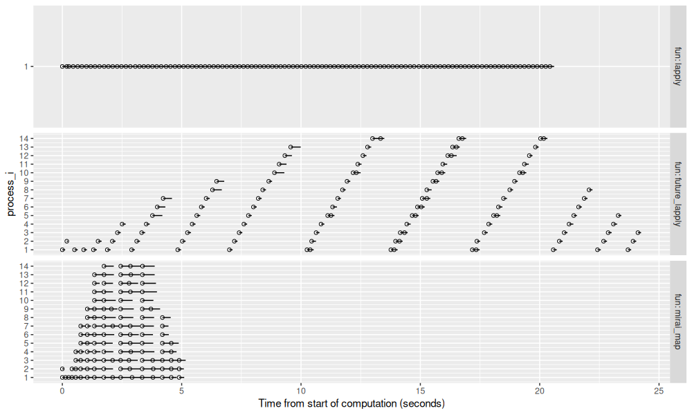
In the figure above, we can see that lapply and future_lapply take
the most time, and mirai_map is much faster (about 5 seconds). This
is an example when mirai_map is particularly advantageous:
- centralized process does not take much time to assign new tasks.
- computation time of each task is relatively small, so overhead of
future_lapplylaunching is relevant.
For longer running computations, for example several minutes or
seconds, there should be smaller differences between future_lapply
and mirai_map.
Parallelization without a central launcher
In this section, we explore the speedups that we can get by using a de-centralized parallel computation, in which each process decides what penalty to compute (there is no central launcher, so one less bottleneck).
Declare some functions
We coordinate the workers using a lock file, in the functions below. The function below creates a new data set directory, and returns the path where we can save model info in an RDS file.
new_data_dir <- function(){
  data.dir <- file.path(
    tempfile(),
    "H3K27ac-H3K4me3_TDHAM_BP",
    "samples",
    "Mono1_H3K27ac",
    "S001YW_NCMLS",
    "problems",
    "chr11-60000-580000")
  dir.create(data.dir, recursive=TRUE, showWarnings=FALSE)
  data(Mono27ac, package="PeakSegDisk")
  write.table(
    Mono27ac$coverage, file.path(data.dir, "coverage.bedGraph"),
    col.names=FALSE, row.names=FALSE, quote=FALSE, sep="\t")
  file.path(data.dir, "summary.rds")
}
The function below attempts to run one new/helpful penalty, based on the models in the RDS file.
Note that we use the filelock R package to
manage a lock file that can guarantee only one process reading/writing this RDS file at a time.
Below we use lock() and unlock() to protect parts of the code where we need to read from the RDS and then write it again.
- in the first lock/unlock block, we read RDS, decide on a new
penvalue to compute, then add a row with that penalty andpeaks=NAto the RDS table. - at this point, if another process looks at the RDS, it will not decide to compute the same
penvalue, because it already exists in the RDS table. - then we compute the model for the new
penvalue viaPeakSegFPOP_dir(). - then in the second lock/unlock block, we read RDS, and save the new
peaksvalue to RDS.
run_penalty <- function(){
  library(data.table)
  data.dir <- dirname(summary.rds)
  lock.file <- paste0(summary.rds, ".LOCK")
  target.max.peaks <- 100
  target.min.peaks <- 1
  lock.obj <- filelock::lock(lock.file)
  start.time.candidates <- Sys.time()
  if(file.exists(summary.rds)){
    task_dt <- readRDS(summary.rds)
    finite_dt <- task_dt[is.finite(peaks)]
  }else{
    finite_dt <- task_dt <- data.table()
  }
  candidates <- if(nrow(finite_dt) < 2){
    c(0, Inf)
  }else{
    selection.df <- penaltyLearning::modelSelection(finite_dt, "total.loss", "peaks")
    selection.dt <- with(selection.df, data.table(
      total.loss,
      min.lambda,
      penalty,
      max.lambda,
      peaks_after=c(peaks[-1],NA),
      peaks
    ))[
      peaks_after<target.max.peaks & peaks>target.min.peaks & peaks_after+1 < peaks,
      max.lambda
    ]
  }
  new.cand <- setdiff(candidates, task_dt$penalty)
  if(length(new.cand)){
    pen <- new.cand[1]
    new_task_dt <- rbind(
      task_dt,
      data.table(
        penalty=pen,
        total.loss=NA_real_,
        process=factor(Sys.getpid()),
        peaks=NA_integer_,
        start.time.candidates,
        end.time.candidates=Sys.time(),
        start.time.model=NA_real_,
        end.time.model=NA_real_))
    saveRDS(new_task_dt, summary.rds)
  }else{
    pen <- NULL
  }
  filelock::unlock(lock.obj)
  if(is.numeric(pen)){
    start.time <- Sys.time()
    fit <- PeakSegDisk::PeakSegFPOP_dir(data.dir, pen)
    end.time <- Sys.time()
    lock.obj <- filelock::lock(lock.file)
    task_dt <- readRDS(summary.rds)
    task_dt[penalty==pen, let(
      total.loss=fit$loss$total.loss,
      peaks=fit$loss$peaks,
      start.time.model=start.time,
      end.time.model=end.time
    )]
    saveRDS(task_dt, summary.rds)
    filelock::unlock(lock.obj)
  }
  pen
}
The code below is the main worker loop of each parallel process. The
function includes a while loop that repeatedly does run_penalty().
If that returns numeric (indicating a model was computed for a new
penalty), then the time is saved. If more than 5 seconds has elapsed
since the last model was computed, then we are done.
run_penalties <- function(seconds.thresh=5){
  done <- FALSE
  last.time <- Sys.time()
  while(!done){
    pen <- run_penalty()
    if(is.numeric(pen)){
      last.time <- Sys.time()
    }
    if(Sys.time()-last.time > seconds.thresh){
      done <- TRUE
    }
  }
}
The function below computes a summary table based on the data in the RDS file.
reshape_summary <- function(){
  (summary_dt <- readRDS(summary.rds))
  nc::capture_melt_multiple(
    summary_dt[, let(
      row = .I,
      process_i = as.integer(process)
    )],
    column=".*", "[.]",
    computation="model|candidates"
  )[, let(
    start.seconds=start.time-min(start.time),
    end.seconds=end.time-min(start.time)
  )][]
}
The function below plots the summary table.
comp.colors <- c(
  model="black",
  candidates="red")
gg_summary <- function(summary_long){
  library(ggplot2)
  ggplot()+
    theme_bw()+
    geom_segment(aes(
      start.seconds, process,
      color=computation,
      xend=end.seconds, yend=process),
      data=summary_long)+
    geom_point(aes(
      start.seconds, process,
      size=computation,
      color=computation),
      shape=1,
      data=summary_long)+
    scale_color_manual(values=comp.colors)+
    scale_size_manual(values=c(
      candidates=3,
      model=2))+
    directlabels::geom_dl(aes(
      start.seconds, process,
      label.group=row,
      label=peaks),
      data=summary_long[computation=="model"],
      method=polygon.mine("bottom", offset.cm=0.2, custom.colors=list(box.color="white")))+
    scale_x_continuous("Time from start of computation (seconds)")
}
Function demo
Below we create a new data directory, then run three penalties.
summary.rds <- new_data_dir()
run_penalty()
## [1] 0
readRDS(summary.rds)
## Indice : <penalty>
##    penalty total.loss process peaks start.time.candidates end.time.candidates start.time.model end.time.model
##      <num>      <num>  <fctr> <int>                <POSc>              <POSc>            <num>          <num>
## 1:       0  -130227.3 1782323  3199   2025-07-04 12:45:41 2025-07-04 12:45:41       1751625941     1751625942
run_penalty()
## [1] Inf
readRDS(summary.rds)
## Indice : <penalty>
##    penalty total.loss process peaks start.time.candidates end.time.candidates start.time.model end.time.model
##      <num>      <num>  <fctr> <int>                <POSc>              <POSc>            <num>          <num>
## 1:       0  -130227.3 1782323  3199   2025-07-04 12:45:41 2025-07-04 12:45:41       1751625941     1751625942
## 2:     Inf   375197.9 1782323     0   2025-07-04 12:45:41 2025-07-04 12:45:41       1751625942     1751625942
run_penalty()
## [1] 157.9947
readRDS(summary.rds)
## Indice : <penalty>
##     penalty total.loss process peaks start.time.candidates end.time.candidates start.time.model end.time.model
##       <num>      <num>  <fctr> <int>                <POSc>              <POSc>            <num>          <num>
## 1:   0.0000 -130227.29 1782323  3199   2025-07-04 12:45:41 2025-07-04 12:45:41       1751625941     1751625942
## 2:      Inf  375197.87 1782323     0   2025-07-04 12:45:41 2025-07-04 12:45:41       1751625942     1751625942
## 3: 157.9947  -62199.93 1782323   224   2025-07-04 12:45:41 2025-07-04 12:45:41       1751625942     1751625942
The tables above show that each call to run_penalty() adds a row with a new penalty value to the RDS file.
The idea is to repeated call this function in many parallel processes.
De-centralized parallelization, lock file, future
Below we use future_lapply() to implement the de-centralized parallel computation.
future::plan("multisession")
summary.rds <- new_data_dir()
null.list <- future.apply::future_lapply(seq(1, parallel::detectCores()), function(i)run_penalties())
summary_future <- reshape_summary()
gg_summary(summary_future)
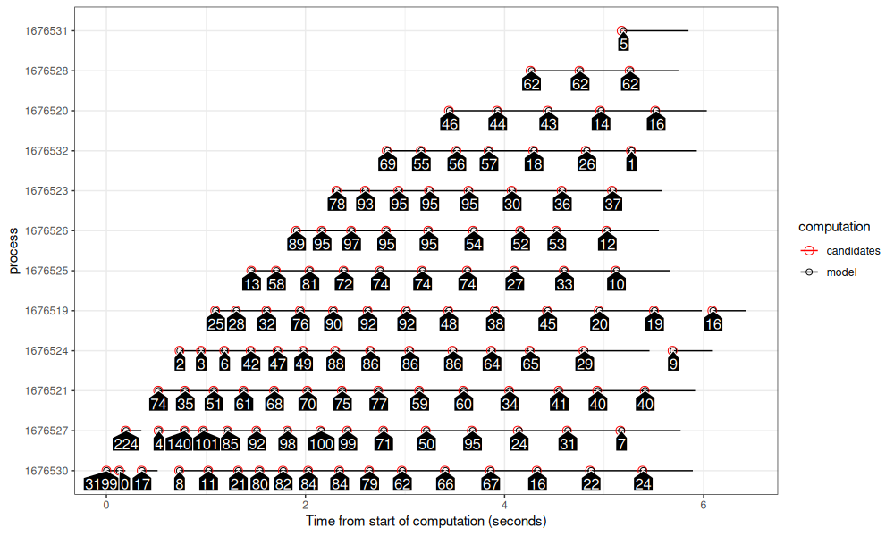
The plot above shows how the parallel computation proceeds over time using future_lapply().
- The first process starts with 3199 peaks at the bottom.
- There is a delay of about 0.2 seconds before starting computation in each other process, as can be seen via the stair step pattern going up to the right.
- With the previous centralized launcher result, when a process finished, it had to wait for the other processes to finish. Then the launcher would assign new work, at which case the process could resume work. Here we see a different pattern: when a computation finishes, a new computation starts almost immediately, with no visible periods where processes have to wait for each other. This reduction of idle time is the main advantage of the de-centralized method of parallelization.
- The computation finishes in about 4 seconds, after each process has decided that there is no more work to do.
De-centralized parallelization, lock file, mirai
Below we use mirai_map() to implement the de-centralized parallel computation.
if(mirai::daemons()$connections==0){
  mirai::daemons(parallel::detectCores())
}
summary.rds <- new_data_dir()
list.of.mirai <- mirai::mirai_map(
  1:parallel::detectCores(),
  function(i)run_penalties(),
  run_penalties=run_penalties,
  run_penalty=run_penalty,
  summary.rds=summary.rds
)[]
summary_mirai <- reshape_summary()
gg_summary(summary_mirai)
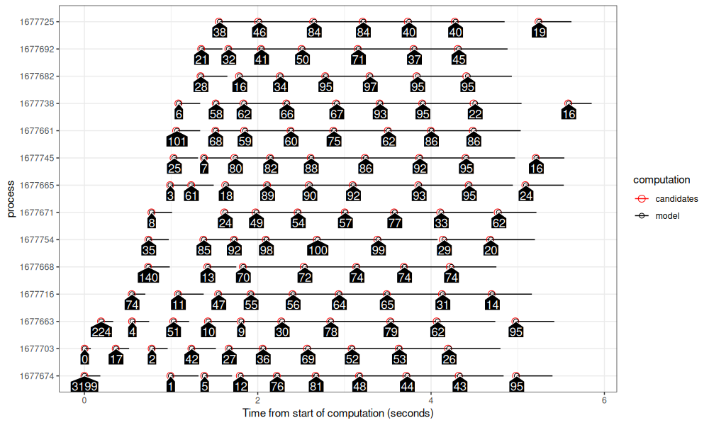
The figure above shows similar patterns as the previous section.
- A less pronounced stair step pattern is evident, because there is a smaller delay between creation of processes.
- There is a somewhat large gap in the bottom left, which is due to the lack of obviously helpful penalties to explore in the beginning of the algorithm.
Comparing de-centralized parallelization packages
The figure below compares the two R functions that we used for de-centralized parallelization.
summary_compare <- rbind(
  data.table(fun="mirai_map", summary_mirai),
  data.table(fun="future_lapply", summary_future))
ggplot()+
  theme_bw()+
  geom_segment(aes(
    start.seconds, process_i,
    color=computation,
    xend=end.seconds, yend=process_i),
    data=summary_compare)+
  geom_point(aes(
    start.seconds, process_i,
    size=computation,
    color=computation),
    shape=1,
    data=summary_compare)+
  scale_color_manual(values=comp.colors)+
  scale_size_manual(values=c(
    candidates=3,
    model=2))+
  scale_y_continuous(breaks=seq(1, parallel::detectCores()))+
  scale_x_continuous("Time from start of computation (seconds)")+
  facet_grid(fun ~ ., labeller=label_both, scales="free", space="free")
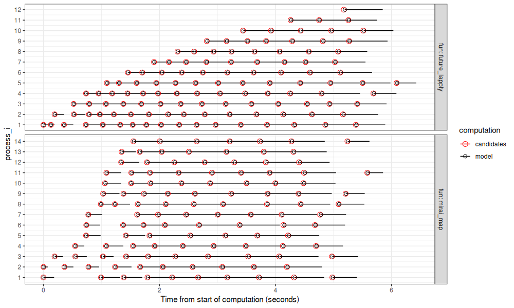
The figure above shows timings on my laptop: mirai_map() is actually a bit slower
than future_lapply() in this case, although the difference is not
large (about 1 second).
Figures below are the same analysis on two Alliance Canada Clusters.
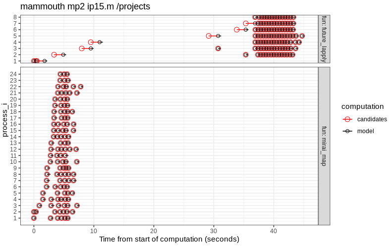
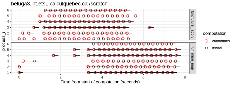
The results above show that:
- the file lock mechanism works on both file systems (/projects and /scratch).
- mirai is much faster than future on
mammouth.
parallel::detectCores()returns 24 on the login node, and this is the number of CPUs used by mirai, but not future. - future is slightly faster than mirai on
beluga.
paralllel::detectCores()returns 40 on the login node, but both frameworks only use 6 CPUs.
Compare everything
The code below combines all timings into a single visualization.
loss_1_100[, let(
  start.seconds=start.time-min(start.time),
  end.seconds=end.time-min(start.time)
)]
common.names <- intersect(names(loss_1_100), names(summary_compare))
all_compare <- rbind(
  data.table(design="de-centralized", summary_compare[computation=="model"][, ..common.names]),
  data.table(design="centralized", loss_1_100[, ..common.names])
)[, Fun := factor(fun, fun_levs)][]
if(FALSE){
  parallelPeaks <- all_compare
  save(parallelPeaks, file="~/R/animint2/data/parallelPeaks.RData")
}
ggplot()+
  theme_bw()+
  geom_segment(aes(
    start.seconds, process_i,
    color=design,
    xend=end.seconds, yend=process_i),
    data=all_compare)+
  geom_point(aes(
    start.seconds, process_i, color=design),
    shape=1,
    data=all_compare)+
  facet_grid(Fun + design ~ ., scales="free", labeller=label_both)+
  scale_y_continuous(breaks=seq(1, parallel::detectCores()))+
  scale_x_continuous("Time from start of computation (seconds)")
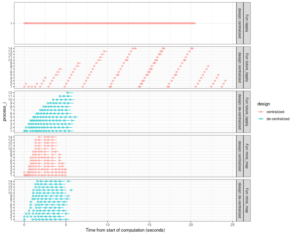
The figure above compares the different parallelization methods we have explored.
- The two methods using
mirai_mapare fast because the delay for launch new processes is very small. - The two methods using de-centralized parallelization are fast because there is no need to wait for a central launcher to assign work. This difference is especially evident when comparing the two
future_lapplymethods.
Conclusions
We have discussed how to implement Change-points for a Range Of ComplexitieS (CROCS), an algorithm that returns a range of peak models. We used a real genomic data set, and computed models with from 1 to 100 peaks. We observed the differences between several computation methods:
lapplysequential computation is relatively slow.future.apply::future_lapplyresults in somewhat faster computation using 14 CPUs on my laptop. The computation time of each job was on the same order of magnitude as the overhead of launching parallel jobs (about 0.2 seconds). For much longer jobs, this overhead is not significant, but for these small jobs, it does result in noticeable slow-downs.mirai::mirai_mapresults in even faster computation, because its overhead is much smaller.- Both functions can be used with de-centralized parallelization,
which greatly reduces computation time using
future_lapplyin this case.
Session Info
sessionInfo()
## R version 4.5.1 (2025-06-13)
## Platform: x86_64-pc-linux-gnu
## Running under: Ubuntu 24.04.2 LTS
##
## Matrix products: default
## BLAS:   /usr/lib/x86_64-linux-gnu/blas/libblas.so.3.12.0
## LAPACK: /usr/lib/x86_64-linux-gnu/lapack/liblapack.so.3.12.0  LAPACK version 3.12.0
##
## locale:
##  [1] LC_CTYPE=fr_FR.UTF-8       LC_NUMERIC=C               LC_TIME=fr_FR.UTF-8        LC_COLLATE=fr_FR.UTF-8
##  [5] LC_MONETARY=fr_FR.UTF-8    LC_MESSAGES=fr_FR.UTF-8    LC_PAPER=fr_FR.UTF-8       LC_NAME=C
##  [9] LC_ADDRESS=C               LC_TELEPHONE=C             LC_MEASUREMENT=fr_FR.UTF-8 LC_IDENTIFICATION=C
##
## time zone: Europe/Paris
## tzcode source: system (glibc)
##
## attached base packages:
## [1] stats     graphics  grDevices datasets  utils     methods   base
##
## other attached packages:
## [1] ggplot2_3.5.2     data.table_1.17.6
##
## loaded via a namespace (and not attached):
##  [1] gtable_0.3.6             future.apply_1.20.0      dplyr_1.1.4              compiler_4.5.1
##  [5] filelock_1.0.3           tidyselect_1.2.1         bspm_0.5.7               parallel_4.5.1
##  [9] dichromat_2.0-0.1        globals_0.18.0           scales_1.4.0             directlabels_2025.5.20
## [13] R6_2.6.1                 labeling_0.4.3           generics_0.1.4           penaltyLearning_2024.9.3
## [17] nanonext_1.6.0           knitr_1.50               backports_1.5.0          redux_1.1.4
## [21] checkmate_2.3.2          future_1.58.0            tibble_3.3.0             mirai_2.3.0
## [25] pillar_1.10.2            RColorBrewer_1.1-3       rlang_1.1.6              xfun_0.52
## [29] quadprog_1.5-8           cli_3.6.5                withr_3.0.2              magrittr_2.0.3
## [33] digest_0.6.37            grid_4.5.1               nc_2025.3.24             PeakSegDisk_2024.10.1
## [37] lifecycle_1.0.4          vctrs_0.6.5              evaluate_1.0.3           glue_1.8.0
## [41] farver_2.1.2             listenv_0.9.1            codetools_0.2-20         parallelly_1.45.0
## [45] tools_4.5.1              pkgconfig_2.0.3
Not working yet
For future work, it would be interesting to compare with these other frameworks.
De-centralized candidate computation, rush
TODO, this is not working, but I asked for help https://github.com/mlr-org/rush/issues/44
data.rush <- file.path(
  tempfile(),
  "H3K27ac-H3K4me3_TDHAM_BP",
  "samples",
  "Mono1_H3K27ac",
  "S001YW_NCMLS",
  "problems",
  "chr11-60000-580000")
dir.create(data.rush, recursive=TRUE, showWarnings=FALSE)
data(Mono27ac,package="PeakSegDisk")
write.table(
  Mono27ac$coverage, file.path(data.rush, "coverage.bedGraph"),
  col.names=FALSE, row.names=FALSE, quote=FALSE, sep="\t")

## rush = rush::RushWorker$new(network_id = "test", config=config, remote=FALSE)
## key = rush$push_running_tasks(list(list(penalty=0)))
## rush$fetch_tasks()
## rush$push_results(key, list(list(peaks=5L, total.loss=5.3)))
## rush$fetch_tasks()
run_penalty <- function(rush){
  target.max.peaks <- 15
  target.min.peaks <- 5
  get_tasks <- function(){
    task_dt <- rush$fetch_tasks()
    if(is.null(task_dt$penalty)){
      task_dt$penalty <- NA_real_
    }
    if(is.null(task_dt$peaks)){
      task_dt$peaks <- NA_integer_
    }
    task_dt
  }
  task_dt <- get_tasks()
  start.time.cand <- Sys.time()
  first_pen_cand <- c(0, Inf)
  done <- first_pen_cand %in% task_dt$penalty
  pen <- if(any(!done)){
    first_pen_cand[!done][1]
  }else{
    print(task_dt)
    while(nrow(task_dt[!is.na(peaks)])<2){
      task_dt <- get_tasks()
    }
    print(task_dt)
    selection.df <- penaltyLearning::modelSelection(task_dt, "total.loss", "peaks")
    selection.dt <- with(selection.df, data.table(
      total.loss,
      min.lambda,
      penalty,
      max.lambda,
      peaks_after=c(peaks[-1],NA),
      peaks
    ))[
      peaks_after<target.max.peaks & peaks>target.min.peaks &
        peaks_after+1 < peaks & !max.lambda %in% task_dt$penalty
    ]
    if(nrow(selection.dt)){
      selection.dt[1, max.lambda]
    }
  }
  if(is.numeric(pen)){
    key = rush$push_running_tasks(xss=list(list(
      penalty=pen,
      start.time.cand=start.time.cand,
      end.time.cand=Sys.time())))
    start.time.model <- Sys.time()
    fit <- PeakSegDisk::PeakSegFPOP_dir(data.rush, pen)
    rush$push_results(key, yss=list(list(
      peaks=fit$loss$peaks,
      total.loss=fit$loss$total.loss,
      start.time.model=start.time.model,
      end.time.model=Sys.time())))
    pen
  }
}
wl_penalty <- function(rush){
  done <- FALSE
  while(!done){
    pen <- run_penalty(rush)
    done <- is.null(pen)
  }
}

if(FALSE){
  redux::hiredis()$pipeline("FLUSHDB")
  config = redux::redis_config()
  rush = rush::Rush$new(network_id = "test", config=config)
  wl_penalty(rush)
  devtools::install_github("mlr-org/rush@mirai")
}


wl_random_search = function(rush) {
  # stop optimization after 100 tasks
  while(rush$n_finished_tasks < 100) {
    # draw new task
    xs = list(x1 = runif(1, -5, 10), x2 = runif(1, 0, 15))
    # mark task as running
    key = rush$push_running_tasks(xss = list(xs))
    # evaluate task
    ys = list(y = branin(xs$x1, xs$x2))
    # push result
    rush$push_results(key, yss = list(ys))
  }
}
branin = function(x1, x2) {
  (x2 - 5.1 / (4 * pi^2) * x1^2 + 5 / pi * x1 - 6)^2 + 10 * (1 - 1 / (8 * pi)) * cos(x1) + 10
}


library(data.table)

redux::hiredis()$pipeline("FLUSHDB")
## [[1]]
## [Redis: OK]
config = redux::redis_config()
rush = rush::Rush$new(network_id = "test", config=config)
rush$fetch_tasks()
## Null data.table (0 rows and 0 cols)
rush$start_local_workers(
  worker_loop = wl_random_search,
  n_workers = 4,
  globals = "branin")
## INFO [12:46:19.904] [rush] Starting 4 worker(s)
rush
## <Rush>
## * Running Workers: 0
## * Queued Tasks: 0
## * Queued Priority Tasks: 0
## * Running Tasks: 0
## * Finished Tasks: 0
## * Failed Tasks: 0
rush$fetch_tasks()
## Null data.table (0 rows and 0 cols)
redux::hiredis()$pipeline("FLUSHDB")
## [[1]]
## [Redis: OK]
config = redux::redis_config()
rush = rush::Rush$new(network_id = "test", config=config)
rush$fetch_tasks()
## Null data.table (0 rows and 0 cols)
rush$start_local_workers(
  worker_loop = wl_penalty,
  n_workers = 4,
  globals = c("run_penalty","data.rush"))
## INFO [12:46:20.233] [rush] Starting 4 worker(s)
rush
## <Rush>
## * Running Workers: 0
## * Queued Tasks: 0
## * Queued Priority Tasks: 0
## * Running Tasks: 0
## * Finished Tasks: 0
## * Failed Tasks: 0
task_dt <- rush$fetch_tasks()
task_dt[order(peaks)]
## Error in .checkTypos(e, names_x): Objet 'peaks' non trouvé parmi []
redis list
TODO code based on redux and transactions or locks?
r <- redux::hiredis()
r$FLUSHDB()
## [Redis: OK]
r$LPUSH()
## Error in r$LPUSH(): l'argument "key" est manquant, avec aucune valeur par défaut