MPI for parallelization in R
The goal of this post is to show how to parallelize machine learning experiments using MPI.
Motivation
This page is similar to another page with an example involving parallel computation of change-point models.
Common code
This code defines the number of CPUs, and number of jobs to compute.
workers <- 10
NCPU <- workers+1
Njob <- 100
work.id.vec <- 1:Njob
The code below defines a function which will be run with one job ID, in different parallel computing frameworks.
job_sleep <- function(work.id){
  library(data.table)
  requireNamespace("pbdMPI") #load to get accurate timing for first job.
  start <- Sys.time()
  my_rank <- tryCatch({
    pbdMPI::comm.rank()
  }, error=function(e)NA_integer_)
  Sys.sleep(work.id/100)
  data.table(my_rank, work.id, start, end=Sys.time(), proc=factor(Sys.getpid()))
}
The function above will sleep/wait for a variable number of seconds (depending on the job ID), and then return a data table of results (including start/end time and process ID).
Be careful: if you are running this code interactively, running job_sleep() will load pbdMPI, which will edit the environment, and then the pbdMPI example system() call below will no longer work.
Below we save the sleep function and initialize a table of timings.
To visualize the results, I coded a special Positioning Method for directlabels::geom_dl.
save(work.id.vec, job_sleep, file="job_sleep.RData")
timing_tables <- list()
diff_seconds <- function(...)as.numeric(difftime(..., units="s"))
polygon.mine <- function
### Make a Positioning Method that places non-overlapping speech
### polygons at the first or last points.
(top.bottom.left.right,
### Character string indicating what side of the plot to label.
  offset.cm=0.1,
### Offset from the polygon to the most extreme data point.
  padding.cm=0.05,
### Padding inside the polygon.
  custom.colors=NULL
### Positioning method applied just before draw.polygons, can set
### box.color and text.color for custom colors.
){
  if(is.null(custom.colors)){
    custom.colors <- directlabels::gapply.fun({
      rgb.mat <- col2rgb(d[["colour"]])
      d$text.color <- with(data.frame(t(rgb.mat)), {
        gray <- 0.3*red + 0.59*green + 0.11*blue
        ifelse(gray/255 < 0.5, "white", "black")
      })
      d
    })
  }
  opposite.side <- c(
    left="right",
    right="left",
    top="bottom",
    bottom="top")[[top.bottom.left.right]]
  direction <- if(
    top.bottom.left.right %in% c("bottom", "left")
  ) -1 else 1
  min.or.max <- if(
    top.bottom.left.right %in% c("top", "right")
  ) max else min
  if(top.bottom.left.right %in% c("left", "right")){
    min.or.max.xy <- "x"
    qp.target <- "y"
    qp.max <- "top"
    qp.min <- "bottom"
    padding.h.factor <- 2
    padding.w.factor <- 1
    limits.fun <- ylimits
    reduce.method <- "reduce.cex.lr"
  }else{
    min.or.max.xy <- "y"
    qp.target <- "x"
    qp.max <- "right"
    qp.min <- "left"
    padding.h.factor <- 1
    padding.w.factor <- 2
    limits.fun <- directlabels::xlimits
    reduce.method <- "reduce.cex.tb"
  }
  list(
    hjust=0.5,
    function(d,...){
      ## set the end of the speech polygon to the original data point.
      for(xy in c("x", "y")){
        extra.coord <- sprintf(# e.g. left.x
          "%s.%s", opposite.side, xy)
        d[[extra.coord]] <- d[[xy]]
      }
      ## offset positions but do NOT set the speech polygon position
      ## to the min or max.
      d[[min.or.max.xy]] <- d[[min.or.max.xy]] + offset.cm*direction
      d
    },
    "calc.boxes",
    reduce.method,
    function(d, ...){
      d$h <- d$h + padding.cm * padding.h.factor
      d$w <- d$w + padding.cm * padding.w.factor
      d
    },
    "calc.borders",
    function(d,...){
      do.call(rbind, lapply(split(d, d$y), function(d){
        directlabels::apply.method(directlabels::qp.labels(
          qp.target,
          qp.min,
          qp.max,
          directlabels::make.tiebreaker(min.or.max.xy, qp.target),
          limits.fun), d)
      }))
    },
    "calc.borders",
    custom.colors,
    "draw.polygons")
}
my.polygons <- list(cex=0.7, vjust=0, polygon.mine(
  "top", offset.cm=0.2, custom.colors=list(box.color="white")))
make_gg <- function(package, expr){
  before <- Sys.time()
  result <- eval(expr)
  if(!is.data.table(result))result <- rbindlist(result)
  after <- Sys.time()
  DT <- data.table(before, after, result)
  timing_tables[[package]] <<- DT
  library(ggplot2)
  rect_dt <- unique(DT[, .(before, after)])
  seconds_possible <- workers*rect_dt[, diff_seconds(after, before)]
  seconds_used <- sum(DT[, diff_seconds(end, start)])
  ggplot()+
    ggtitle(sprintf("%s efficiency = %.1f%%", package, 100*seconds_used/seconds_possible))+
    theme_bw()+
    geom_rect(aes(
      xmin=before, xmax=after,
      ymin = -Inf, ymax=Inf),
      data=rect_dt,
      alpha=0.5,
      fill="grey")+
    geom_segment(aes(
      start, proc,
      xend=end, yend=proc),
      data=DT)+
    geom_point(aes(
      start, proc),
      shape=1,
      data=DT)+
    directlabels::geom_dl(aes(
      start, proc,
      label.group=paste(work.id, proc),
      label=work.id),
      data=DT,
      method=my.polygons)+
    scale_x_continuous("Time (seconds)")
}
library(data.table)
mirai code
In R we can use the code below to ask mirai to do the scheduling using processes on the local computer:
mirai::daemons(NULL)
## [1] 0
mirai::daemons(workers)
## [1] 10
make_gg("mirai", mirai::mirai_map(work.id.vec, job_sleep)[])
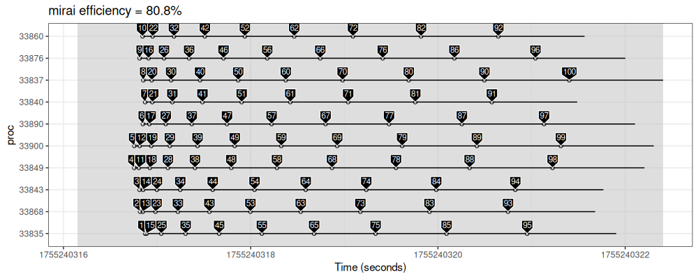
We see in the figure above that there are 3 processes (Y axis ticks), and 10 jobs (labels and segments).
future code
Another way to do it in R is using future package for scheduling:
future::plan("multisession", workers=workers)
make_gg("future", future.apply::future_lapply(work.id.vec, job_sleep))
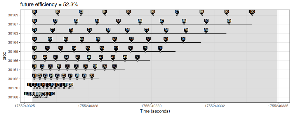
The figure above shows similar trends, but with a noticeable delay between processes, and some idle time in the first process (static scheduling).
pbdMPI code
Another way to do it in R is via MPI, using the pbdMPI package:
script_sleep <- function(prefix){
  code <- gsub("SCRIPT", prefix, 'library(data.table)
load("SCRIPT_sleep.RData")
ret_dt_list <- pbdMPI::task.pull(work.id.vec, SCRIPT_sleep)
ret_dt <- rbindlist(ret_dt_list)
if(pbdMPI::comm.rank() == 0)fwrite(ret_dt, "SCRIPT_sleep.csv")
pbdMPI::finalize()
')
  sleep.R <- paste0(prefix, "_sleep.R")
  cat(code, file=sleep.R)
  cmd <- sprintf("mpiexec -np %d Rscript --vanilla %s", NCPU, sleep.R)
  sleep.csv <- paste0(prefix, "_sleep.csv")
  unlink(sleep.csv)
  system(cmd)
  fread(sleep.csv, colClasses=list(factor="proc"))
}
Note in the code above we have used mpiexec to run Rscript with a certain number of CPUs (-np argument).
In the context of a SLURM compute cluster, we can substitute mpiexec -np 4 with srun, which will use MPI with -np set to the number of tasks in the job (sbatch --ntasks).
This is the approach we use in mlr3resampling::proj_submit().
make_gg("pbdMPI", script_sleep("job"))
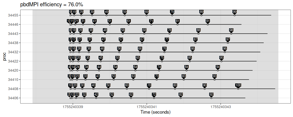
The figure above shows that the pbdMPI scheduling is more efficient than future, but also static (nearby jobs are assigned to different processes).
Compare
In this section, we combine results from the different packages.
add_seconds <- function(DT, sec.cols = c("start","end","before","after"))DT[
, paste0(sec.cols, ".seconds") :=
    lapply(sec.cols, function(x)diff_seconds(get(x), before))
]
(compare_dt <- data.table(package=names(timing_tables))[
, add_seconds(timing_tables[[package]])
, by=package])
##      package              before               after my_rank work.id               start                 end   proc
##       <char>              <POSc>              <POSc>   <int>   <int>              <POSc>              <POSc> <fctr>
##   1:   mirai 2025-08-15 02:45:16 2025-08-15 02:45:22       0       1 2025-08-15 02:45:16 2025-08-15 02:45:16  33835
##   2:   mirai 2025-08-15 02:45:16 2025-08-15 02:45:22       0       2 2025-08-15 02:45:16 2025-08-15 02:45:16  33868
##   3:   mirai 2025-08-15 02:45:16 2025-08-15 02:45:22       0       3 2025-08-15 02:45:16 2025-08-15 02:45:16  33843
##   4:   mirai 2025-08-15 02:45:16 2025-08-15 02:45:22       0       4 2025-08-15 02:45:16 2025-08-15 02:45:16  33849
##   5:   mirai 2025-08-15 02:45:16 2025-08-15 02:45:22       0       5 2025-08-15 02:45:16 2025-08-15 02:45:16  33900
##  ---
## 296:  pbdMPI 2025-08-15 02:45:37 2025-08-15 02:45:44       6      96 2025-08-15 02:45:43 2025-08-15 02:45:44  34432
## 297:  pbdMPI 2025-08-15 02:45:37 2025-08-15 02:45:44       7      97 2025-08-15 02:45:43 2025-08-15 02:45:44  34438
## 298:  pbdMPI 2025-08-15 02:45:37 2025-08-15 02:45:44       8      98 2025-08-15 02:45:43 2025-08-15 02:45:44  34443
## 299:  pbdMPI 2025-08-15 02:45:37 2025-08-15 02:45:44      10      99 2025-08-15 02:45:43 2025-08-15 02:45:44  34455
## 300:  pbdMPI 2025-08-15 02:45:37 2025-08-15 02:45:44       2     100 2025-08-15 02:45:43 2025-08-15 02:45:44  34408
##      start.seconds end.seconds before.seconds after.seconds
##              <num>       <num>          <num>         <num>
##   1:     0.7211623   0.7315655              0      6.256604
##   2:     0.6676934   0.6884851              0      6.256604
##   3:     0.6616662   0.6920228              0      6.256604
##   4:     0.6051404   0.6457052              0      6.256604
##   5:     0.6060286   0.6564395              0      6.256604
##  ---
## 296:     5.1984246   6.1593895              0      6.651924
## 297:     5.2816756   6.2523866              0      6.651924
## 298:     5.3742917   6.3553576              0      6.651924
## 299:     5.4642127   6.4544086              0      6.651924
## 300:     5.5620975   6.5627975              0      6.651924
rect_dt <- unique(compare_dt[, .(package, before.seconds, after.seconds)])
ggplot()+
  theme_bw()+
  geom_blank(aes(
    -Inf, ""),
    data=unique(compare_dt[, .(package)]))+
  geom_rect(aes(
    xmin=before.seconds, xmax=after.seconds,
    ymin = -Inf, ymax=Inf),
    data=rect_dt,
    alpha=0.5,
    fill="grey")+
  geom_segment(aes(
    start.seconds, proc,
    xend=end.seconds, yend=proc),
    data=compare_dt)+
  geom_point(aes(
    start.seconds, proc),
    shape=1,
    data=compare_dt)+
  directlabels::geom_dl(aes(
    start.seconds, proc,
    label.group=paste(work.id, proc),
    label=work.id),
    data=compare_dt,
    method=my.polygons)+
  facet_grid(package ~ ., labeller=label_both, scales="free")+
  scale_y_discrete("process")+
  scale_x_continuous(
    "Seconds since line before apply",
    limits=c(0, NA))
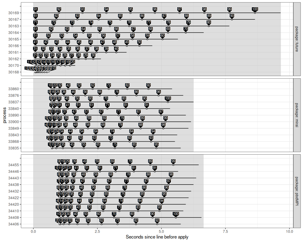
The figure above shows a pretty substantial difference: future uses static scheduling (first ten jobs on first processor, etc), and pbdMPI seems to as well (first ten jobs are assigned to run first on the ten CPUs, etc), whereas mirai is dynamic (each processor asks for a new job from a queue).
Although the MPI approach is slightly less efficient than mirai in this simple example, it is more easily usable on a SLURM cluster.
Furthermore, the MPI approach can be used to overcome the limitations of batchtools:
- whereas
batchtoolsuses one job array task, and one CPU, per work ID, - dynamic scheduling with MPI allows treatment of heterogeneous work (with different time requirements),
- and multiple CPUs can be used per job (which can help mitigate the max 1000 SLURM job limit imposed by Alliance Canada).
Similar in python
See torc_py.
Another pbdMPI example
In this example, we sleep based on the process rank, instead of the job ID.
rank_sleep <- function(work.id){
  library(data.table)
  requireNamespace("pbdMPI") #load to get accurate timing for first job.
  start <- Sys.time()
  my_rank <- pbdMPI::comm.rank()
  Sys.sleep(my_rank/10)
  data.table(rank=my_rank, work.id, start, end=Sys.time(), proc=factor(Sys.getpid()))
}
save(work.id.vec, rank_sleep, file="rank_sleep.RData")
rank_dt <- script_sleep("rank")
ggplot()+
  theme_bw()+
  geom_segment(aes(
    start, rank,
    xend=end, yend=rank),
    data=rank_dt)+
  geom_point(aes(
    start, rank),
    shape=1,
    data=rank_dt)+
  directlabels::geom_dl(aes(
    start, rank,
    label.group=paste(work.id, rank),
    label=work.id),
    data=rank_dt,
    method=my.polygons)+
  scale_y_continuous(breaks=1:workers, limits=c(1, NCPU))+
  scale_x_continuous("Time (seconds)")
![]()
The figure above shows that the pbdMPI scheduling is in fact dynamic – larger ranks process only a few job IDs, whereas smaller ranks do quite a lot of work.
Conclusions
We have shown how to do parallel computations in R using several frameworks: mirai, future, and MPI.
These functions can be useful for parallelizing machine learning experiments.
In practice to use MPI to launch machine learning benchmarks, I recommend using mlr3resampling::proj_submit().
Session info
sessionInfo()
## R version 4.5.1 (2025-06-13)
## Platform: x86_64-pc-linux-gnu
## Running under: Ubuntu 24.04.2 LTS
##
## Matrix products: default
## BLAS:   /usr/lib/x86_64-linux-gnu/blas/libblas.so.3.12.0
## LAPACK: /usr/lib/x86_64-linux-gnu/lapack/liblapack.so.3.12.0  LAPACK version 3.12.0
##
## locale:
##  [1] LC_CTYPE=fr_FR.UTF-8       LC_NUMERIC=C               LC_TIME=fr_FR.UTF-8        LC_COLLATE=fr_FR.UTF-8
##  [5] LC_MONETARY=fr_FR.UTF-8    LC_MESSAGES=fr_FR.UTF-8    LC_PAPER=fr_FR.UTF-8       LC_NAME=C
##  [9] LC_ADDRESS=C               LC_TELEPHONE=C             LC_MEASUREMENT=fr_FR.UTF-8 LC_IDENTIFICATION=C
##
## time zone: America/Toronto
## tzcode source: system (glibc)
##
## attached base packages:
## [1] stats     graphics  grDevices datasets  utils     methods   base
##
## other attached packages:
## [1] ggplot2_3.5.2     data.table_1.17.8
##
## loaded via a namespace (and not attached):
##  [1] directlabels_2025.6.24 vctrs_0.6.5            cli_3.6.5              knitr_1.50             rlang_1.1.6
##  [6] xfun_0.52              generics_0.1.4         glue_1.8.0             nanonext_1.6.2         labeling_0.4.3
## [11] mirai_2.4.1            future.apply_1.20.0    listenv_0.9.1          scales_1.4.0           quadprog_1.5-8
## [16] grid_4.5.1             evaluate_1.0.4         tibble_3.3.0           lifecycle_1.0.4        compiler_4.5.1
## [21] codetools_0.2-20       dplyr_1.1.4            RColorBrewer_1.1-3     pkgconfig_2.0.3        future_1.67.0
## [26] digest_0.6.37          farver_2.1.2           R6_2.6.1               dichromat_2.0-0.1      tidyselect_1.2.1
## [31] parallelly_1.45.1      parallel_4.5.1         pillar_1.11.0          magrittr_2.0.3         tools_4.5.1
## [36] withr_3.0.2            gtable_0.3.6           globals_0.18.0         bspm_0.5.7