Speed of named versus numbered indexing in R
The goal of this post is to explore the source of a recent
issue that was fixed
in animint2, my R package for animated interactive data
visualization.
Motivation: Hi-C data
PhD student Elise JORGE from INRAE Touloue is currently visiting my lab at Sherbrooke. We are working on methods for clustering, analysis, and visualization of Hi-C data.
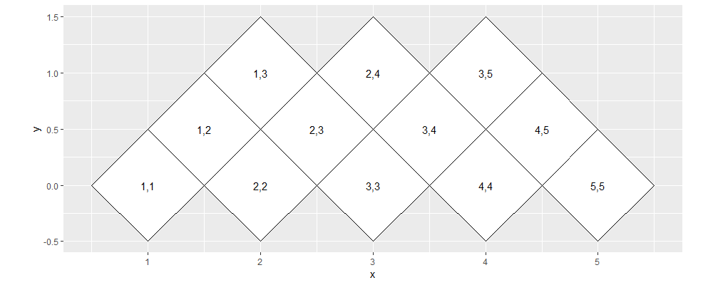
Visualizing example data with tiles
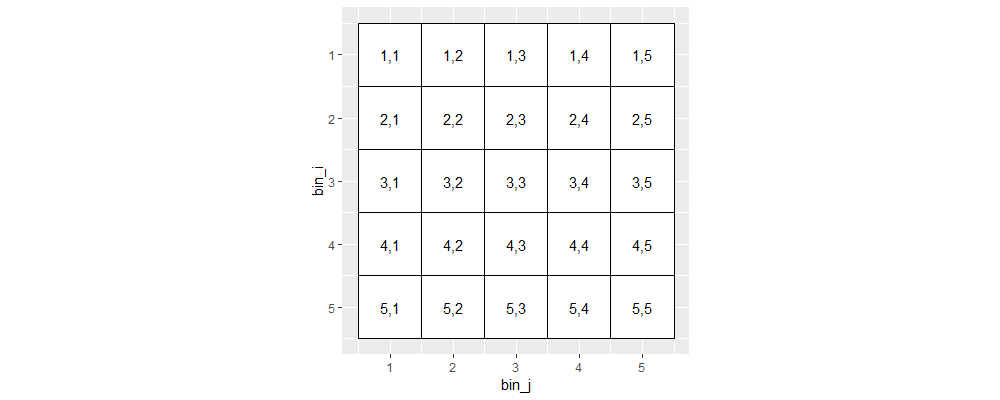
In R, those data can be represented as a pairwise interaction matrix or data table, where each interacting element is a bin in genomic position space.
library(data.table)
N_bins <- 5
bin_vec <- seq(1, N_bins)
(ij_dt <- CJ(
  bin_i=bin_vec,
  bin_j=bin_vec
)[, label := sprintf("%d,%d", bin_i, bin_j)])
library(ggplot2)
ggplot()+
  coord_equal()+
  geom_tile(aes(
    bin_j, bin_i),
    color="black",
    fill="white",
    data=ij_dt)+
  geom_text(aes(
    bin_j, bin_i, label=label),
    data=ij_dt)+
  scale_y_reverse()
There are integer read counts associated with each bin pair (i,j), which are symmetric (same for j,i), so we typically visualize only half of the data.
(ij_half <- ij_dt[bin_i <= bin_j])
## Key: <bin_i, bin_j>
##     bin_i bin_j  label
##     <int> <int> <char>
##  1:     1     1    1,1
##  2:     1     2    1,2
##  3:     1     3    1,3
##  4:     1     4    1,4
##  5:     1     5    1,5
##  6:     2     2    2,2
##  7:     2     3    2,3
##  8:     2     4    2,4
##  9:     2     5    2,5
## 10:     3     3    3,3
## 11:     3     4    3,4
## 12:     3     5    3,5
## 13:     4     4    4,4
## 14:     4     5    4,5
## 15:     5     5    5,5
ggplot()+
  coord_equal()+
  geom_tile(aes(
    bin_j, bin_i),
    color="black",
    fill="white",
    data=ij_half)+
  geom_text(aes(
    bin_j, bin_i, label=label),
    data=ij_half)+
  scale_y_reverse()
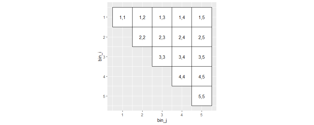
Above we see the lower triangle has been removed. Furthermore, we typically visualize only close-range interactions.
(ij_close <- ij_half[bin_j <= bin_i + 2])
## Key: <bin_i, bin_j>
##     bin_i bin_j  label
##     <int> <int> <char>
##  1:     1     1    1,1
##  2:     1     2    1,2
##  3:     1     3    1,3
##  4:     2     2    2,2
##  5:     2     3    2,3
##  6:     2     4    2,4
##  7:     3     3    3,3
##  8:     3     4    3,4
##  9:     3     5    3,5
## 10:     4     4    4,4
## 11:     4     5    4,5
## 12:     5     5    5,5
ggplot()+
  coord_equal()+
  geom_tile(aes(
    bin_j, bin_i),
    color="black",
    fill="white",
    data=ij_close)+
  geom_text(aes(
    bin_j, bin_i, label=label),
    data=ij_close)+
  scale_y_reverse()
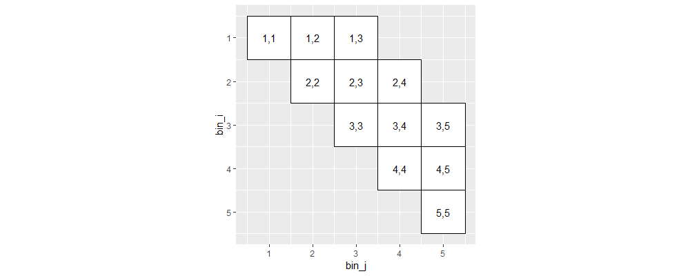
Above we see that long-range interactions have been removed (upper right of plot).
Visualizing using polygons
To visualize these typically rotate 45 degrees, so that the diagonal of the matrix goes from left to right. To do that we first convert i,j coordinates to corners, which we draw using polygons in the code below.
(corner_dt <- setkey(ij_close[, data.table(
  bin_i=rep(bin_i, 4),
  bin_j=rep(bin_j, 4),
  label=rep(label, 4),
  corner_i=c(bin_i-0.5, bin_i-0.5, bin_i+0.5, bin_i+0.5),
  corner_j=c(bin_j-0.5, bin_j+0.5, bin_j+0.5, bin_j-0.5)
)], label))
## Key: <label>
##     bin_i bin_j  label corner_i corner_j
##     <int> <int> <char>    <num>    <num>
##  1:     1     1    1,1      0.5      0.5
##  2:     1     1    1,1      0.5      1.5
##  3:     1     1    1,1      1.5      1.5
##  4:     1     1    1,1      1.5      0.5
##  5:     1     2    1,2      0.5      1.5
##  6:     1     2    1,2      0.5      2.5
##  7:     1     2    1,2      1.5      2.5
##  8:     1     2    1,2      1.5      1.5
##  9:     1     3    1,3      0.5      2.5
## 10:     1     3    1,3      0.5      3.5
## 11:     1     3    1,3      1.5      3.5
## 12:     1     3    1,3      1.5      2.5
## 13:     2     2    2,2      1.5      1.5
## 14:     2     2    2,2      1.5      2.5
## 15:     2     2    2,2      2.5      2.5
## 16:     2     2    2,2      2.5      1.5
## 17:     2     3    2,3      1.5      2.5
## 18:     2     3    2,3      1.5      3.5
## 19:     2     3    2,3      2.5      3.5
## 20:     2     3    2,3      2.5      2.5
## 21:     2     4    2,4      1.5      3.5
## 22:     2     4    2,4      1.5      4.5
## 23:     2     4    2,4      2.5      4.5
## 24:     2     4    2,4      2.5      3.5
## 25:     3     3    3,3      2.5      2.5
## 26:     3     3    3,3      2.5      3.5
## 27:     3     3    3,3      3.5      3.5
## 28:     3     3    3,3      3.5      2.5
## 29:     3     4    3,4      2.5      3.5
## 30:     3     4    3,4      2.5      4.5
## 31:     3     4    3,4      3.5      4.5
## 32:     3     4    3,4      3.5      3.5
## 33:     3     5    3,5      2.5      4.5
## 34:     3     5    3,5      2.5      5.5
## 35:     3     5    3,5      3.5      5.5
## 36:     3     5    3,5      3.5      4.5
## 37:     4     4    4,4      3.5      3.5
## 38:     4     4    4,4      3.5      4.5
## 39:     4     4    4,4      4.5      4.5
## 40:     4     4    4,4      4.5      3.5
## 41:     4     5    4,5      3.5      4.5
## 42:     4     5    4,5      3.5      5.5
## 43:     4     5    4,5      4.5      5.5
## 44:     4     5    4,5      4.5      4.5
## 45:     5     5    5,5      4.5      4.5
## 46:     5     5    5,5      4.5      5.5
## 47:     5     5    5,5      5.5      5.5
## 48:     5     5    5,5      5.5      4.5
##     bin_i bin_j  label corner_i corner_j
ggplot()+
  coord_equal()+
  geom_polygon(aes(
    corner_j, corner_i, group=label),
    color="black",
    fill="white",
    data=corner_dt)+
  geom_text(aes(
    bin_j, bin_i, label=label),
    data=ij_close)+
  scale_y_reverse()
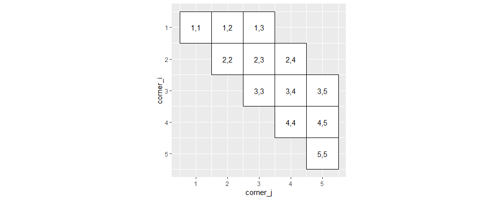
The plot above using polygons is consistent with previous plots that use tiles. Next, we compute a rotation matrix which converts ij-coordinates to xy-coordinates.
two.ij <- rbind(
  c(1,1),
  c(1,2))
two.xy <- rbind(
  c(1,   0),  #i,j=1,1 maps to x,y=1,0
  c(1.5, 0.5))#i,j=1,2 maps to x,y=1.5,0.5
(ij2xy_mat <- solve(two.ij) %*% two.xy)
##      [,1] [,2]
## [1,]  0.5 -0.5
## [2,]  0.5  0.5
Below we verify that the linear transformation matrix ij2xy_mat works as intended, for the two ij-vectors used in the solve() (matrix inverse):
corner_dt[, two.ij %*% ij2xy_mat]
##      [,1] [,2]
## [1,]  1.0  0.0
## [2,]  1.5  0.5
The output above is same matrix as two.xy, as expected.
Next, we use the tranformation ij2xy_mat on all of the ij coordinates (corners and bins):
setxy <- function(DT, prefix){
  ij_mat <- as.matrix(DT[, sprintf("%s_%s",prefix,c("i","j")), with=FALSE])
  DT[, c("x","y") := as.data.table(ij_mat %*% ij2xy_mat)]
}
setxy(corner_dt, "corner")[1:8]
## Key: <label>
##    bin_i bin_j  label corner_i corner_j     x     y
##    <int> <int> <char>    <num>    <num> <num> <num>
## 1:     1     1    1,1      0.5      0.5   0.5   0.0
## 2:     1     1    1,1      0.5      1.5   1.0   0.5
## 3:     1     1    1,1      1.5      1.5   1.5   0.0
## 4:     1     1    1,1      1.5      0.5   1.0  -0.5
## 5:     1     2    1,2      0.5      1.5   1.0   0.5
## 6:     1     2    1,2      0.5      2.5   1.5   1.0
## 7:     1     2    1,2      1.5      2.5   2.0   0.5
## 8:     1     2    1,2      1.5      1.5   1.5   0.0
setxy(ij_close, "bin")[1:2]
## Key: <bin_i, bin_j>
##    bin_i bin_j  label     x     y
##    <int> <int> <char> <num> <num>
## 1:     1     1    1,1   1.0   0.0
## 2:     1     2    1,2   1.5   0.5
The output tables above have additional columns with xy-coordinates, which are plotted below.
ggplot()+
  coord_equal()+
  geom_polygon(aes(
    x, y, group=label),
    fill="white",
    color="black",
    data=corner_dt)+
  geom_text(aes(
    x, y, label=label),
    data=ij_close)
Above we see that the polygons have been rotated 45 degrees, such that the diagonal is now at y=0.
Exploring time complexity
The animint2 package has a sophisticated compiler, that tries to compress data in each geom, before writing CSV files that will be read by the JavaScript code for visualization.
For geom_polygon, and others which have aes(group), the code loops over each group, looking for common data across subsets.
The old code split the data table into a list of tables, one per group, as below.
list_of_dt <- split(corner_dt, corner_dt$label)[1:2]
Then there was a loop over names of this list, as below.
for(element_name in names(list_of_dt)){
  list_of_dt[[element_name]]
}
The code above uses named lookup, which I suspect is responsible for the quadratic time complexity we observed.
Test for loop
To test this hypothesis, we use the code below.
ares <- atime::atime(
  setup={
    N_list <- structure(as.list(1:N), names=1:N)
  },
  name=for(name in names(N_list))N_list[[name]],
  index=for(index in seq_along(N_list))N_list[[index]])
plot(ares)
## Warning in ggplot2::scale_y_log10("median line, min/max band"): log-10 transformation introduced infinite values.
## log-10 transformation introduced infinite values.
## log-10 transformation introduced infinite values.
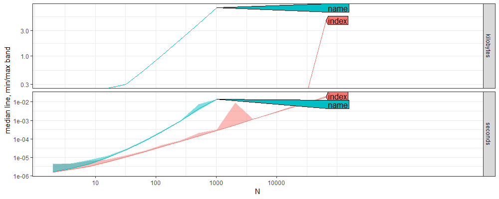
The plot above shows asymptotic time and memory measurements for looping through a list, using either names or indices.
We see in the seconds panel that the name method has a larger slope than the index method, which suggests a larger computational complexity class.
Below we estimate the asymptotic complexity of each method.
aref <- atime::references_best(ares)
plot(aref)
## Warning in ggplot2::scale_y_log10(""): log-10 transformation introduced infinite values.
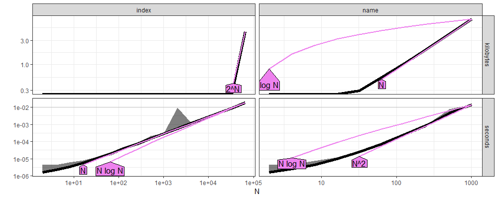
Above we see the empirical measurements in black, with asymptotic references in violet.
indexis clearly linear,O(N).nameis clearly quadratic,O(N^2).
These data confirm the hypothesis that the slowdown in the old code was caused by the loop over the groups in which we used lookup by name (not index).
The different complexity classes are consistent with the performance test case we created in order to ensure that we maintain linear time complexity for this operation in animint2 (link to result in PR that added the performance test).
Finally, the code below estimates the throughput for each method.
apred <- predict(aref)
plot(apred)
## Warning in ggplot2::scale_x_log10("N", breaks = meas[, 10^seq(ceiling(min(log10(N))), : log-10 transformation introduced infinite values.
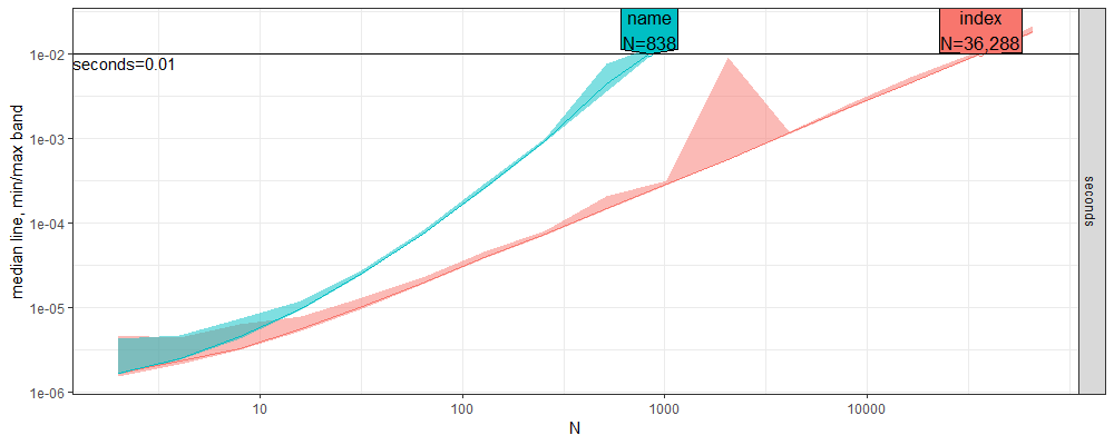
The figure above shows that the throughput of index-based lookup is about 50x larger than named-based lookup, for the default time limit of 0.01 seconds. In the real data, there are 100k groups or more, which can explain the slowdown with the previous quadratic time code.
Test without for loop
We should be able to see differences without the for loop. A single list lookup should be
- linear time with a name,
- constant time with a number.
The code below runs the corresponding test.
atime_one <- atime::atime(
  setup={
    N_vec <- structure(1:N, names=1:N)
    N_chr <- as.character(N)
  },
  name_1=N_vec[["1"]],
  name_N=N_vec[[N_chr]],
  index_N=N_vec[[N]])
plot(atime_one)
## Warning in ggplot2::scale_y_log10("median line, min/max band"): log-10 transformation introduced infinite values.
## log-10 transformation introduced infinite values.
## log-10 transformation introduced infinite values.
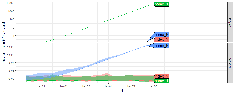
The figure above shows time and memory usage as a function of N, the size of the vector.
index_N, index access of the last element, is constant time,O(1).name_1, name access of the first element, is constant time,O(1).name_N, name access of the last element, is linear time,O(N).
Conclusions
This post has explored the time complexity of list lookup in R.
- Because name-based list lookup uses a linear scan of names, each lookup is a linear time operation, and a loop over all elements is quadratic time.
- Each index-based list lookup is constant time, and a loop over all elements is linear time.
This suggests that a simple fix for the issue would have been to use indices rather than names for the list lookup.
The solution we adopted was porting the code to data.table and using by instead of a loop, which has the same effect (linear time overall because data are sorted prior to looping over groups).
Session info
sessionInfo()
## R version 4.4.1 (2024-06-14 ucrt)
## Platform: x86_64-w64-mingw32/x64
## Running under: Windows 11 x64 (build 26100)
##
## Matrix products: default
##
##
## locale:
## [1] LC_COLLATE=English_United States.utf8  LC_CTYPE=English_United States.utf8    LC_MONETARY=English_United States.utf8
## [4] LC_NUMERIC=C                           LC_TIME=English_United States.utf8
##
## time zone: America/Toronto
## tzcode source: internal
##
## attached base packages:
## [1] stats     graphics  utils     datasets  grDevices methods   base
##
## other attached packages:
## [1] ggplot2_3.5.1      data.table_1.16.99
##
## loaded via a namespace (and not attached):
##  [1] directlabels_2024.1.21 vctrs_0.6.5            knitr_1.48             cli_3.6.3              xfun_0.47              rlang_1.1.4
##  [7] highr_0.11             bench_1.1.3            generics_0.1.3         glue_1.7.0             labeling_0.4.3         colorspace_2.1-1
## [13] scales_1.3.0           fansi_1.0.6            quadprog_1.5-8         grid_4.4.1             evaluate_0.24.0        munsell_0.5.1
## [19] tibble_3.2.1           profmem_0.6.0          lifecycle_1.0.4        compiler_4.4.1         dplyr_1.1.4            pkgconfig_2.0.3
## [25] atime_2025.5.24        farver_2.1.2           lattice_0.22-6         R6_2.5.1               tidyselect_1.2.1       utf8_1.2.4
## [31] pillar_1.9.0           magrittr_2.0.3         tools_4.4.1            withr_3.0.1            gtable_0.3.5