Comparing neural network architectures using mlr3torch
The goal of this blog is to demonstrate improvements in prediction accuracy using neural networks, compared to linear models, for image classification tasks, using mlr3torch in R.
Introduction
A major advantage of the mlr3torch framework in R, is that it is relatively simple to compare different learning algorithms, on different data sets, in terms of prediction accuracy in cross-validation. For example, in a previous post, we showed that a torch linear model with early stopping regularization is slightly but significantly more accurate than an L1-regularized linear model, for image classification.
The goal here is to reproduce the results similar to figures in my Two New Algos slides, which show that convolutional neural networks are more accurate than linear models in image classification.
Read MNIST data
We begin by reading the MNIST data,
library(data.table)
## data.table 1.17.0 utilise 7 threads (voir ?getDTthreads).  Dernières actualités : r-datatable.com
## **********
## Running data.table in English; package support is available in English only. When searching for online help, be sure to also check for the English error message. This can be obtained by looking at the po/R-<locale>.po and po/<locale>.po files in the package source, where the native language and English error messages can be found side-by-side. You can also try calling Sys.setLanguage('en') prior to reproducing the error message.
## **********
MNIST_dt <- fread("~/projects/cv-same-other-paper/data_Classif/MNIST.csv")
dim(MNIST_dt)
## [1] 70000 786
data.table(
  name=names(MNIST_dt),
  first_row=unlist(MNIST_dt[1]),
  last_row=unlist(MNIST_dt[.N]))
##                name first_row last_row
##              <char>    <char>   <char>
##   1: predefined.set     train     test
##   2:              y         5        6
##   3:              0         0        0
##   4:              1         0        0
##   5:              2         0        0
##  ---
## 782:            779         0        0
## 783:            780         0        0
## 784:            781         0        0
## 785:            782         0        0
## 786:            783         0        0
We then create a label factor column, and a task:
MNIST_dt[, label := factor(y)]
mtask <- mlr3::TaskClassif$new(
  "MNIST", MNIST_dt, target="label")
mtask$col_roles$stratum <- "label"
mtask$col_roles$feature <- grep("^[0-9]+$", names(MNIST_dt), value=TRUE)
mtask
## <TaskClassif:MNIST> (70000 x 785)
## * Target: label
## * Properties: multiclass, strata
## * Features (784):
##   - dbl (784): 0, 1, 10, 100, 101, 102, 103, 104, 105, 106, 107, 108, 109, 11, 110, 111, 112, 113, 114,
##     115, 116, 117, 118, 119, 12, 120, 121, 122, 123, 124, 125, 126, 127, 128, 129, 13, 130, 131, 132, 133,
##     134, 135, 136, 137, 138, 139, 14, 140, 141, 142, 143, 144, 145, 146, 147, 148, 149, 15, 150, 151, 152,
##     153, 154, 155, 156, 157, 158, 159, 16, 160, 161, 162, 163, 164, 165, 166, 167, 168, 169, 17, 170, 171,
##     172, 173, 174, 175, 176, 177, 178, 179, 18, 180, 181, 182, 183, 184, 185, 186, 187, 188, [...]
## * Strata: label
The Task above is the mlr3 representation of the MNIST data set with the meta-data about which columns should be used for input/output/stratum/etc.
Defining neural network architecture
We can use the function below to define neural networks with the same learning rate, step size, etc, but different architecture (number of hidden layers/units).
measure_list <- mlr3::msrs(c("classif.logloss", "classif.ce"))
n.epochs <- 200
make_torch_learner <- function(id,...){
  po_list <- c(
    list(
      mlr3pipelines::po(
        "select",
        selector = mlr3pipelines::selector_type(c("numeric", "integer"))),
      mlr3torch::PipeOpTorchIngressNumeric$new()),
    list(...),
    list(
      mlr3pipelines::po("nn_head"),
      mlr3pipelines::po(
        "torch_loss",
        mlr3torch::t_loss("cross_entropy")),
      mlr3pipelines::po(
        "torch_optimizer",
        mlr3torch::t_opt("sgd", lr=0.1)),
      mlr3pipelines::po(
        "torch_callbacks",
        mlr3torch::t_clbk("history")),
      mlr3pipelines::po(
        "torch_model_classif",
        batch_size = 100,
        patience=n.epochs,
        measures_valid=measure_list,
        measures_train=measure_list,
        predict_type="prob",
        epochs = paradox::to_tune(upper = n.epochs, internal = TRUE)))
    )
    graph <- Reduce(mlr3pipelines::concat_graphs, po_list)
    glearner <- mlr3::as_learner(graph)
    mlr3::set_validate(glearner, validate = 0.5)
    mlr3tuning::auto_tuner(
      learner = glearner,
      tuner = mlr3tuning::tnr("internal"),
      resampling = mlr3::rsmp("insample"),
      measure = mlr3::msr("internal_valid_score", minimize = TRUE),
      term_evals = 1,
      id=id,
      store_models = TRUE)
}
The function above has a variable number of inputs:
- the first argument is a
learner_idto display in the results. - the other arguments are used to define the neural network
architecture, after torch ingress numeric, and before
nn_head, which is mlr3torch terminology for the last layer of the neural network (output size determined by the task).
The code below defines a list of learners:
n.pixels <- 28
learner.list <- list(
  make_torch_learner("torch_linear"),
  make_torch_learner(
    "torch_dense_50",
    mlr3pipelines::po(
      "nn_linear",
      out_features = 50),
    mlr3pipelines::po("nn_relu_1", inplace = TRUE)
  ),
  make_torch_learner(
    "torch_conv",
    mlr3pipelines::po(
      "nn_reshape",
      shape=c(-1,1,n.pixels,n.pixels)),
    mlr3pipelines::po(
      "nn_conv2d_1",
      out_channels = 20,
      kernel_size = 6),
    mlr3pipelines::po("nn_relu_1", inplace = TRUE),
    mlr3pipelines::po(
      "nn_max_pool2d_1",
      kernel_size = 4),
    mlr3pipelines::po("nn_flatten"),
    mlr3pipelines::po(
      "nn_linear",
      out_features = 50),
    mlr3pipelines::po("nn_relu_2", inplace = TRUE)
  ),
  mlr3::LearnerClassifFeatureless$new()$configure(id="featureless"),
  mlr3learners::LearnerClassifCVGlmnet$new()$configure(id="cv_glmnet")
)
The code above uses make_torch_learner three times:
torch_linearcreates a linear model (one layer of parameters to learn). Even with no architecture arguments, thenn_headgenerates a linear layer which is compatible with the inputs and outputs.torch_dense_50creates a neural network with one hidden layer, of 50 hidden units, followed by ReLU activation (two layers of parameters to learn).torch_convcreates a neural network with a 2D convolution, followed by ReLU activation, followed by 2D max pooling, followed by a flatten operation and a linear layer, then a final ReLU (three layers of parameters to learn).
Defining and computing a benchmark grid
The code below combines the task, learners, and a resampling method (3-fold cross-validation), in a benchmark grid:
kfoldcv <- mlr3::rsmp("cv")
kfoldcv$param_set$values$folds <- 3
(bench.grid <- mlr3::benchmark_grid(
  mtask,
  learner.list,
  kfoldcv))
##      task        learner resampling
##    <char>         <char>     <char>
## 1:  MNIST   torch_linear         cv
## 2:  MNIST torch_dense_50         cv
## 3:  MNIST     torch_conv         cv
## 4:  MNIST    featureless         cv
## 5:  MNIST      cv_glmnet         cv
The code below does the computation.
reg.dir <- "2025-03-20-mlr3torch-conv"
cache.RData <- paste0(reg.dir,".RData")
if(file.exists(cache.RData)){
  load(cache.RData)
}else{
  if(FALSE){#code below only works on the cluster.
    unlink(reg.dir, recursive=TRUE)
    reg = batchtools::makeExperimentRegistry(
      file.dir = reg.dir,
      seed = 1,
      packages = "mlr3verse"
    )
    mlr3batchmark::batchmark(
      bench.grid, store_models = TRUE, reg=reg)
    job.table <- batchtools::getJobTable(reg=reg)
    chunks <- data.frame(job.table, chunk=1)
    batchtools::submitJobs(chunks, resources=list(
      walltime = 60*60,#seconds
      memory = 2000,#megabytes per cpu
      ncpus=1,  #>1 for multicore/parallel jobs.
      ntasks=1, #>1 for MPI jobs.
      chunks.as.arrayjobs=TRUE), reg=reg)
    batchtools::getStatus(reg=reg)
    jobs.after <- batchtools::getJobTable(reg=reg)
    table(jobs.after$error)
    ids <- jobs.after[is.na(error), job.id]
    bench.result <- mlr3batchmark::reduceResultsBatchmark(ids, reg = reg)
  }else{
    ## In the code below, we declare a multisession future plan to
    ## compute each benchmark iteration in parallel on this computer
    ## (data set, learning algorithm, cross-validation fold). For a
    ## few dozen iterations, using the multisession backend is
    ## probably sufficient (I have 12 CPUs on my work PC).
    if(require(future))plan("multisession")
    bench.result <- mlr3::benchmark(bench.grid, store_models = TRUE)
  }
  save(bench.result, file=cache.RData)
}
The code above took several hours on my 14-core laptop.
Test error results
First, we use score() to compute test error rates:
score_dt <- bench.result$score()
(score_some <- score_dt[order(classif.ce), .(
  learner_id=factor(learner_id, unique(learner_id)),
  iteration,
  percent_error=100*classif.ce)])
##         learner_id iteration percent_error
##             <fctr>     <int>         <num>
##  1:     torch_conv         1      1.114158
##  2:     torch_conv         2      1.285733
##  3:     torch_conv         3      1.341563
##  4: torch_dense_50         1      2.901097
##  5: torch_dense_50         2      2.905756
##  6: torch_dense_50         3      2.983155
##  7:   torch_linear         3      7.445030
##  8:   torch_linear         2      7.812969
##  9:   torch_linear         1      7.974803
## 10:      cv_glmnet         2      8.078687
## 11:      cv_glmnet         1      9.770312
## 12:      cv_glmnet         3     10.102439
## 13:    featureless         2     88.745554
## 14:    featureless         1     88.747000
## 15:    featureless         3     88.748875
The table above has one row for each learning algorithm, and each train/test split in 3-fold CV (iteration). It is sorted by error rate, so it is easy to see that the convolutional network is most accurate, and all algorithms have smaller test error rates than featureless. Below we visualize these test error rates in a figure:
library(ggplot2)
ggplot()+
  geom_point(aes(
    percent_error, learner_id),
    shape=1,
    data=score_some)+
  scale_x_continuous(
    breaks=seq(0,100,by=10),
    limits=c(0,90))
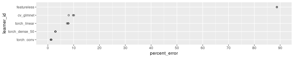
The figure above shows a dot for each learning algorithm and
train/test split. The algorithms on the Y axis are sorted by error
rate, so it is easy to see that torch_conv has the smallest error
rate, the torch_dense_50 has slightly larger error rate,
etc. Interestingly, the torch_linear model (early stopping
regularization) has a slightly smaller error rate than cv_glmnet
(linear model with L1 regularization).
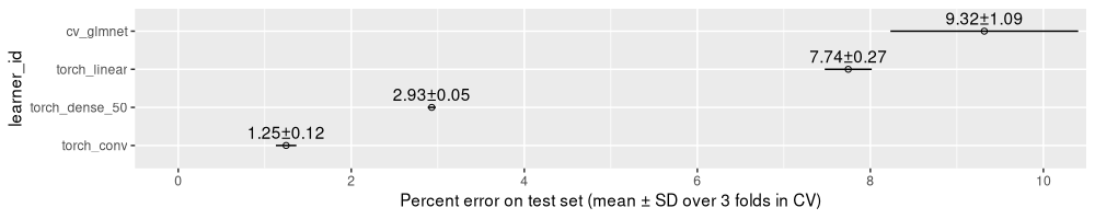
Below we compute mean and standard deviation for each learning algorithm, across the three cross-validation splits:
(score_stats <- dcast(
  score_some,
  learner_id ~ .,
  list(mean, sd),
  value.var="percent_error"))
## Key: <learner_id>
##        learner_id percent_error_mean percent_error_sd
##            <fctr>              <num>            <num>
## 1:     torch_conv           1.247151      0.118509820
## 2: torch_dense_50           2.930003      0.046090490
## 3:   torch_linear           7.744267      0.271486073
## 4:      cv_glmnet           9.317146      1.085316841
## 5:    featureless          88.747143      0.001665273
The table above has one row for each learning algorithm, and columns for mean and standard deviation of the error rate. We visualize these numbers in the figure below:
score_show <- score_stats[learner_id!="featureless"]
ggplot()+
  geom_point(aes(
    percent_error_mean, learner_id),
    shape=1,
    data=score_show)+
  geom_segment(aes(
    percent_error_mean+percent_error_sd, learner_id,
    xend=percent_error_mean-percent_error_sd, yend=learner_id),
    data=score_show)+
  geom_text(aes(
    percent_error_mean, learner_id,
    label=sprintf("%.2f±%.2f", percent_error_mean, percent_error_sd)),
    vjust=-0.5,
    data=score_show)+
  coord_cartesian(xlim=c(0,10))+
  scale_x_continuous(
    "Percent error on test set (mean ± SD over 3 folds in CV)",
    breaks=seq(0,10,by=2))
The figure above omits featureless, to emphasize the subtle differences between the non-trivial learning algorithms. To compute p-values for differences, we can do the following.
(levs <- levels(score_some$learner_id))
## [1] "torch_conv" "torch_dense_50" "torch_linear" "cv_glmnet" "featureless"
(pval_dt <- data.table(comparison_i=1:3)[, {
  two_levs <- levs[comparison_i+c(0,1)]
  lev2rank <- structure(c("lo","hi"), names=two_levs)
  i_long <- score_some[
    learner_id %in% two_levs
  ][
  , rank := lev2rank[paste(learner_id)]
  ][]
  i_wide <- dcast(i_long, iteration ~ rank, value.var="percent_error")
  paired <- with(i_wide, t.test(lo, hi, alternative = "l", paired=TRUE))
  unpaired <- with(i_wide, t.test(lo, hi, alternative = "l", paired=FALSE))
  data.table(
    learner.lo=factor(two_levs[1],levs),
    learner.hi=factor(two_levs[2],levs),
    p.paired=paired$p.value,
    p.unpaired=unpaired$p.value,
    mean.diff=paired$est,
    mean.lo=unpaired$est[1],
    mean.hi=unpaired$est[2])
}, by=comparison_i])
##    comparison_i     learner.lo     learner.hi     p.paired   p.unpaired mean.diff  mean.lo  mean.hi
##           <int>         <fctr>         <fctr>        <num>        <num>     <num>    <num>    <num>
## 1:            1     torch_conv torch_dense_50 0.0004843437 0.0002299919 -1.682852 1.247151 2.930003
## 2:            2 torch_dense_50   torch_linear 0.0007180091 0.0003970101 -4.814265 2.930003 7.744267
## 3:            3   torch_linear      cv_glmnet 0.0767237001 0.0606614992 -1.572879 7.744267 9.317146
The table above has one row for each comparison, with columns for mean error rates and P-values (in paired and unpaired T-tests). These P-values are shown in the figure below.
ggplot()+
  geom_segment(aes(
    mean.lo, learner.lo,
    xend=mean.hi, yend=learner.lo),
    data=pval_dt,
    size=2,
    color="red")+
  geom_text(aes(
    x=(mean.lo+mean.hi)/2, learner.lo,
    label=sprintf("P=%.4f", p.paired)),
    data=pval_dt,
    vjust=1.5,
    color="red")+
  geom_point(aes(
    percent_error_mean, learner_id),
    shape=1,
    data=score_show)+
  geom_segment(aes(
    percent_error_mean+percent_error_sd, learner_id,
    xend=percent_error_mean-percent_error_sd, yend=learner_id),
    size=1,
    data=score_show)+
  geom_text(aes(
    percent_error_mean, learner_id,
    label=sprintf("%.2f±%.2f", percent_error_mean, percent_error_sd)),
    vjust=-0.5,
    data=score_show)+
  coord_cartesian(xlim=c(0,10))+
  scale_y_discrete("algorithm")+
  scale_x_continuous(
    "Percent error on test set (mean ± SD over 3 folds in CV)",
    breaks=seq(0,10,by=2))
## Warning: Using `size` aesthetic for lines was deprecated in ggplot2 3.4.0.
## ℹ Please use `linewidth` instead.
## This warning is displayed once every 8 hours.
## Call `lifecycle::last_lifecycle_warnings()` to see where this warning was generated.
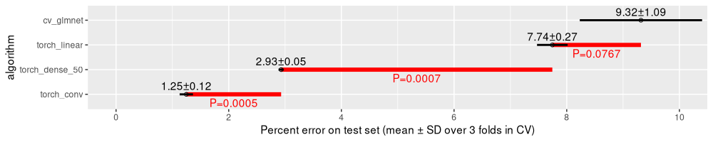
The plot above contains P-values in red, which show that
- the dense neural network has a significantly larger error rate than the convolutional neural network,
- the torch linear model has a significantly larger error rate than the dense neural network,
- the
cv_glmnetlinear model has slightly larger error rate than the torch linear model, but this difference is not statistically significant (at least using the classic threshold of P=0.05).
Checking subtrain/validation loss curves
Next, we can check if we have used enough epochs for the early stopping regularization in torch. If we have used enough, we should see the min validation loss at an intermediate value, not at the smallest number of epochs (underfitting), nor at the largest number of epochs (overfitting). First, we extract the number of epochs that was used by mlr3 auto-tuner, for the torch learners:
(score_torch <- score_dt[
  grepl("torch",learner_id)
][
, best_epoch := sapply(
  learner, function(L)unlist(L$tuning_result$internal_tuned_values))
][])
##       nr task_id     learner_id resampling_id iteration     prediction_test classif.ce best_epoch
##    <int>  <char>         <char>        <char>     <int>              <list>      <num>      <int>
## 1:     1   MNIST     torch_conv            cv         1 <PredictionClassif> 0.01114158         26
## 2:     1   MNIST     torch_conv            cv         2 <PredictionClassif> 0.01285733         23
## 3:     1   MNIST     torch_conv            cv         3 <PredictionClassif> 0.01341563         23
## 4:     2   MNIST   torch_linear            cv         1 <PredictionClassif> 0.07974803         64
## 5:     2   MNIST   torch_linear            cv         2 <PredictionClassif> 0.07812969         78
## 6:     2   MNIST   torch_linear            cv         3 <PredictionClassif> 0.07445030         75
## 7:     4   MNIST torch_dense_50            cv         1 <PredictionClassif> 0.02901097         46
## 8:     4   MNIST torch_dense_50            cv         2 <PredictionClassif> 0.02905756         51
## 9:     4   MNIST torch_dense_50            cv         3 <PredictionClassif> 0.02983155         41
## Hidden columns: uhash, task, learner, resampling
The table above has a best_epoch column which shows the number of epochs that was chosen by the mlr3 auto-tuner.
Next, we extract the history that was used to select the best epoch:
(history_torch <- score_torch[, {
  L <- learner[[1]]
  M <- L$archive$learners(1)[[1]]$model
  M$torch_model_classif$model$callbacks$history
}, by=.(learner_id, iteration)])
##           learner_id iteration epoch train.classif.logloss train.classif.ce valid.classif.logloss valid.classif.ce
##               <char>     <int> <num>                 <num>            <num>                 <num>            <num>
##    1:     torch_conv         1     1           0.799753396       0.24455683            0.27249253       0.08464769
##    2:     torch_conv         1     2           0.195132621       0.05786045            0.19175192       0.06111778
##    3:     torch_conv         1     3           0.133706889       0.04054517            0.13374945       0.03925939
##    4:     torch_conv         1     4           0.106475045       0.03227327            0.09840952       0.02841591
##    5:     torch_conv         1     5           0.091334409       0.02764444            0.09336915       0.02880165
##   ---
## 1796: torch_dense_50         3   196           0.002287684       0.00000000            0.16825939       0.03612599
## 1797: torch_dense_50         3   197           0.002275216       0.00000000            0.16776731       0.03646882
## 1798: torch_dense_50         3   198           0.002244204       0.00000000            0.16788841       0.03616885
## 1799: torch_dense_50         3   199           0.002235485       0.00000000            0.16813258       0.03625455
## 1800: torch_dense_50         3   200           0.002215431       0.00000000            0.16815445       0.03655453
The table above has one row for each learner, iteration, and epoch of training. There are columns named train/valid logloss/ce, which we convert from wide to long format below:
(history_long <- nc::capture_melt_single(
  history_torch,
  set=nc::alevels(valid="validation", train="subtrain"),
  ".classif.",
  measure=nc::alevels("logloss", ce="prop_error")))
##           learner_id iteration epoch        set    measure      value
##               <char>     <int> <num>     <fctr>     <fctr>      <num>
##    1:     torch_conv         1     1   subtrain    logloss 0.79975340
##    2:     torch_conv         1     2   subtrain    logloss 0.19513262
##    3:     torch_conv         1     3   subtrain    logloss 0.13370689
##    4:     torch_conv         1     4   subtrain    logloss 0.10647505
##    5:     torch_conv         1     5   subtrain    logloss 0.09133441
##   ---
## 7196: torch_dense_50         3   196 validation prop_error 0.03612599
## 7197: torch_dense_50         3   197 validation prop_error 0.03646882
## 7198: torch_dense_50         3   198 validation prop_error 0.03616885
## 7199: torch_dense_50         3   199 validation prop_error 0.03625455
## 7200: torch_dense_50         3   200 validation prop_error 0.03655453
The table above has a set column that is consistent with the Deep Learning book of Goodfellow:
- The full data set is split into train and test sets,
- and then the train set is split into subtrain and validation sets.
The code below can be used to visualize the logistic loss for each epoch:
ggplot()+
  theme_bw()+
  theme(legend.position=c(0.9, 0.15))+
  geom_vline(aes(
    xintercept=best_epoch),
    data=score_torch)+
  geom_text(aes(
    best_epoch, Inf, label=paste0(" best epoch=", best_epoch)),
    vjust=1.5, hjust=0,
    data=score_torch)+
  geom_line(aes(
    epoch, value, color=set),
    data=history_long[measure=="logloss"])+
  facet_grid(iteration ~ learner_id, labeller=label_both)+
  scale_y_log10("logistic loss")+
  scale_x_continuous("epoch")
## Warning: A numeric `legend.position` argument in `theme()` was deprecated in ggplot2 3.5.0.
## ℹ Please use the `legend.position.inside` argument of `theme()` instead.
## This warning is displayed once every 8 hours.
## Call `lifecycle::last_lifecycle_warnings()` to see where this warning was generated.
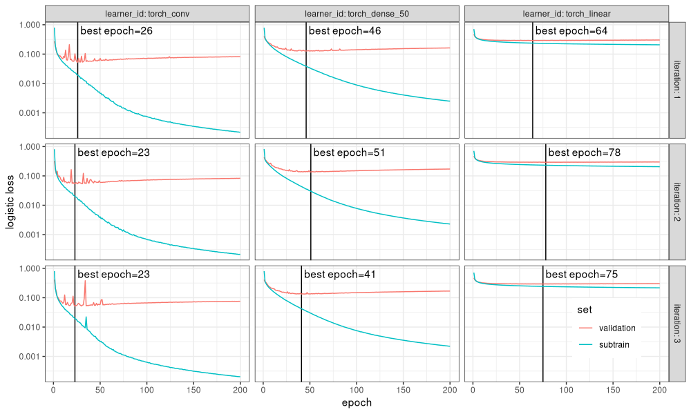
The figure above shows
- panels from left to right for different learning algorithms (neural network architectures),
- panels from top to bottom for different train/test splits in cross-validation (iteration in mlr3 terms),
- Y axis on the log scale to emphasize subtle differences. For example it is clear that the subtrain loss gets much smaller for the convolutional model, than for the dense/linear models.
- a vertical black line in each panel to indicate the best epoch used by the mlr3 auto-tuner. It is clear that this is the min of the validation loss.
The code below considers only the first train/test split in cross-validation, and shows the classification error in addition to the log loss:
get_fold <- function(DT,it=1)DT[iteration==it]
history_fold <- get_fold(history_long)
score_fold <- get_fold(score_torch)
min_fold <- history_fold[
, .SD[value==min(value)]
, by=.(learner_id, measure, set)
][, point := "min"]
ggplot()+
  theme_bw()+
  theme(legend.position=c(0.9, 0.2))+
  geom_vline(aes(
    xintercept=best_epoch),
    data=score_fold)+
  geom_text(aes(
    best_epoch, Inf, label=paste0(" best epoch=", best_epoch)),
    vjust=1.5, hjust=0,
    data=score_fold)+
  geom_line(aes(
    epoch, value, color=set),
    data=history_fold)+
  geom_point(aes(
    epoch, value, color=set, fill=point),
    shape=21,
    data=min_fold)+
  scale_fill_manual(values=c(min="black"))+
  facet_grid(measure ~ learner_id, labeller=label_both, scales="free")+
  scale_x_continuous("epoch")+
  scale_y_log10("")
## Warning in scale_y_log10(""): log-10 transformation introduced infinite values.
## log-10 transformation introduced infinite values.
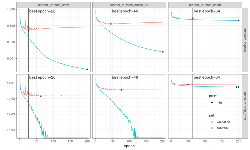
The figure above additionally has black dots to emphasize the minima of each curve. It is clear that the vertical black line (best number of epochs from mlr3 auto-tuner) agrees with the min validation loss (black dot computed using min of each history curve). Finally, we see that the neural networks overfit with perfect classification accuracy on the subtrain set (black dots at bottom of panel), whereas the linear model subtrain error rate never goes below 1%.
Conclusions
We have explained how to use mlr3torch to compare various neural network architectures for image classification, on the MNIST data set. We showed how to code figures that compare test error rates, and allow to check if the max number of epochs was selected appropriately. We saw that a convolutional neural network with three layers of weights was more accurate than a dense neural network with two layers of weights, which was in turn more accurate than a linear model with only one layer of weights. Using a learning rate of 0.1 and a batch size of 100, we saw that 200 epochs was sufficient to observe overfitting, and also to avoid underfitting.
Session info
sessionInfo()
## R version 4.5.0 (2025-04-11)
## Platform: x86_64-pc-linux-gnu
## Running under: Ubuntu 24.04.2 LTS
##
## Matrix products: default
## BLAS:   /usr/lib/x86_64-linux-gnu/blas/libblas.so.3.12.0
## LAPACK: /usr/lib/x86_64-linux-gnu/lapack/liblapack.so.3.12.0  LAPACK version 3.12.0
##
## locale:
##  [1] LC_CTYPE=fr_FR.UTF-8       LC_NUMERIC=C               LC_TIME=fr_FR.UTF-8        LC_COLLATE=fr_FR.UTF-8
##  [5] LC_MONETARY=fr_FR.UTF-8    LC_MESSAGES=fr_FR.UTF-8    LC_PAPER=fr_FR.UTF-8       LC_NAME=C
##  [9] LC_ADDRESS=C               LC_TELEPHONE=C             LC_MEASUREMENT=fr_FR.UTF-8 LC_IDENTIFICATION=C
##
## time zone: Europe/Paris
## tzcode source: system (glibc)
##
## attached base packages:
## [1] stats     graphics  grDevices utils     datasets  methods   base
##
## other attached packages:
## [1] ggplot2_3.5.1     data.table_1.17.0
##
## loaded via a namespace (and not attached):
##  [1] future_1.34.0        generics_0.1.3       listenv_0.9.1        digest_0.6.37        magrittr_2.0.3
##  [6] evaluate_1.0.3       grid_4.5.0           processx_3.8.6       backports_1.5.0      mlr3learners_0.10.0
## [11] torch_0.14.2         ps_1.9.0             scales_1.3.0         coro_1.1.0           mlr3_0.23.0
## [16] mlr3tuning_1.3.0     codetools_0.2-20     mlr3measures_1.0.0   palmerpenguins_0.1.1 cli_3.6.5
## [21] rlang_1.1.6          crayon_1.5.3         parallelly_1.43.0    bit64_4.6.0-1        munsell_0.5.1
## [26] withr_3.0.2          nc_2025.3.24         mlr3pipelines_0.7.2  tools_4.5.0          parallel_4.5.0
## [31] uuid_1.2-1           checkmate_2.3.2      dplyr_1.1.4          colorspace_2.1-1     globals_0.16.3
## [36] bbotk_1.5.0          vctrs_0.6.5          R6_2.6.1             lifecycle_1.0.4      bit_4.6.0
## [41] mlr3misc_0.16.0      pkgconfig_2.0.3      callr_3.7.6          pillar_1.10.2        gtable_0.3.6
## [46] glue_1.8.0           Rcpp_1.0.14          lgr_0.4.4            paradox_1.0.1        xfun_0.51
## [51] tibble_3.2.1         tidyselect_1.2.1     knitr_1.50           farver_2.1.2         labeling_0.4.3
## [56] compiler_4.5.0       mlr3torch_0.2.1-9000