Are pipe operations linear or quadratic?
The goal of this post is to explain how to use atime, my R package for asymptotic benchmarking, to determine the asymptotic complexity of pipe operations in mlr3.
Background: mlr3pipelines man page
mlr3 is a framework for machine learning in R. One related package is
mlr3pipelines, which makes it easy to create “pipelines” of operations
related to machine learning model training (feature selection,
etc). To create a pipeline we use the %>>% operator; its documentation on
help("%>>%",package="mlr3pipelines") says
%>>% always creates deep copies of its input arguments, so they
cannot be modified by reference afterwards. To access individual
‘PipeOp’s after composition, use the resulting ‘Graph’'s $pipeops
list. %>>!%, on the other hand, tries to avoid cloning its first
argument: If it is a ‘Graph’, then this ‘Graph’ will be modified
in-place.

When %>>!% fails, then it leaves ‘g1’ in an incompletely modified
state. It is therefore usually recommended to use %>>%, since the
very marginal gain of performance from using %>>!% often does not
outweigh the risk of either modifying objects by-reference that
should not be modified or getting graphs that are in an
incompletely modified state. However, when creating long ‘Graph’s,
chaining with %>>!% instead of %>>% can give noticeable
performance benefits because %>>% makes a number of
‘clone()’-calls that is quadratic in chain length, %>>!% only
linear.
The man page above indicates that there are two operators which can be used to create a pipeline:
%>>%copies its arguments and is supposed to be quadratic time,%>>!%avoids copies and is supposed to be linear time.
The goal of this post is to use atime to verify these claims.
Test
First we list available pipe ops:
mlr3pipelines::po()
## <DictionaryPipeOp> with 72 stored values
## Keys: adas, blsmote, boxcox, branch, chunk, classbalancing, classifavg, classweights, colapply,
##   collapsefactors, colroles, copy, datefeatures, encode, encodeimpact, encodelmer, featureunion, filter,
##   fixfactors, histbin, ica, imputeconstant, imputehist, imputelearner, imputemean, imputemedian,
##   imputemode, imputeoor, imputesample, kernelpca, learner, learner_cv, learner_pi_cvplus,
##   learner_quantiles, missind, modelmatrix, multiplicityexply, multiplicityimply, mutate, nearmiss, nmf,
##   nop, ovrsplit, ovrunite, pca, proxy, quantilebin, randomprojection, randomresponse, regravg,
##   removeconstants, renamecolumns, replicate, rowapply, scale, scalemaxabs, scalerange, select, smote,
##   smotenc, spatialsign, subsample, targetinvert, targetmutate, targettrafoscalerange, textvectorizer,
##   threshold, tomek, tunethreshold, unbranch, vtreat, yeojohnson
Below, we combine a few instances of the first operation shown above:
po_list <- list(
  mlr3pipelines::po("adas_1"),
  mlr3pipelines::po("adas_2"))
Reduce(mlr3pipelines::`%>>%`, po_list)
## Graph with 2 PipeOps:
##      ID         State sccssors prdcssors
##  <char>        <char>   <char>    <char>
##  adas_1 <<UNTRAINED>>   adas_2
##  adas_2 <<UNTRAINED>>             adas_1
Reduce(mlr3pipelines::`%>>!%`, po_list)
## Graph with 2 PipeOps:
##      ID         State sccssors prdcssors
##  <char>        <char>   <char>    <char>
##  adas_1 <<UNTRAINED>>   adas_2
##  adas_2 <<UNTRAINED>>             adas_1
We see above that the two results are consistent. Note that we use
Reduce with a list of pipe operations, to avoid attaching,
library(mlr3pipelines) (easier to see which objects are defined in
which packages).
Verification
One way to test would be to use binary operators, as below:
FUN_names <- paste0("%>>",c("","!"),"%")
FUN_list <- lapply(FUN_names, getFromNamespace, "mlr3pipelines")
names(FUN_list) <- FUN_names
(expr.list.binary <- atime::atime_grid(
  list(FUN=FUN_names),
  binary=Reduce(FUN_list[[FUN]], po_list)))
## $`binary FUN=%>>!%`
## Reduce(FUN_list[["%>>!%"]], po_list)
##
## $`binary FUN=%>>%`
## Reduce(FUN_list[["%>>%"]], po_list)
##
## attr(,"parameters")
##           expr.name expr.grid    FUN
##              <char>    <char> <char>
## 1: binary FUN=%>>!%    binary  %>>!%
## 2:  binary FUN=%>>%    binary   %>>%
Another way would be to use the concat_graphs function, as below:
(expr.list.concat <- atime::atime_grid(
  list(in_place=c(TRUE,FALSE)),
  concat=Reduce(
    function(x,y)mlr3pipelines::concat_graphs(x,y,in_place=in_place),
    po_list)))
## $`concat in_place=FALSE`
## Reduce(function(x, y) mlr3pipelines::concat_graphs(x, y, in_place = FALSE),
##     po_list)
##
## $`concat in_place=TRUE`
## Reduce(function(x, y) mlr3pipelines::concat_graphs(x, y, in_place = TRUE),
##     po_list)
##
## attr(,"parameters")
##                expr.name expr.grid in_place
##                   <char>    <char>   <lgcl>
## 1: concat in_place=FALSE    concat    FALSE
## 2:  concat in_place=TRUE    concat     TRUE
We can test both by combining the lists in the code below:
atime_list <- atime::atime(
  setup={
    po_list <- lapply(
      paste0("adas_", 1:N),
      mlr3pipelines::po)
  },
  expr.list=c(expr.list.binary, expr.list.concat),
  seconds.limit=1)
## Warning: Some expressions had a GC in every iteration; so filtering is disabled.
## Warning: Some expressions had a GC in every iteration; so filtering is disabled.
## Warning: Some expressions had a GC in every iteration; so filtering is disabled.
plot(atime_list)+
  ggplot2::scale_x_log10(
    breaks=2^seq(1,5),
    limits=c(2,100))
## Scale for x is already present.
## Adding another scale for x, which will replace the existing scale.
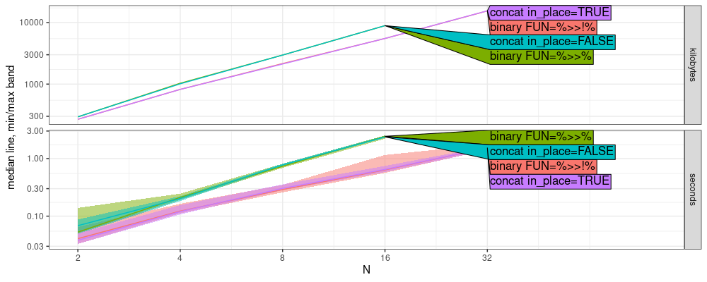
From the figure above, we see that there are two different slopes on the log-log plot:
binary FUN=%>>%andconcat in_place=FALSEhave larger slope.binary FUN=%>>!%andconcat in_place=TRUEhave smaller slope.
We estimate the asymptotic complexity class via the code below,
atime_refs <- atime::references_best(atime_list)
plot(atime_refs)
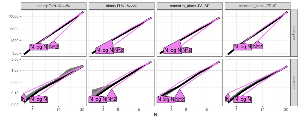
The figure above suggests that
binary FUN=%>>%andconcat in_place=FALSEhave quadraticN^2time complexitybinary FUN=%>>!%andconcat in_place=TRUEhave linearNtime complexity,
where N is the number of operations in the pipeline.
Conclusions
We have used atime to verify the linear/quadratic time complexity claims in the mlr3pipelines package.
Session info
sessionInfo()
## R Under development (unstable) (2025-02-06 r87694)
## Platform: x86_64-pc-linux-gnu
## Running under: Ubuntu 22.04.5 LTS
##
## Matrix products: default
## BLAS:   /usr/lib/x86_64-linux-gnu/blas/libblas.so.3.10.0
## LAPACK: /usr/lib/x86_64-linux-gnu/lapack/liblapack.so.3.10.0  LAPACK version 3.10.0
##
## locale:
##  [1] LC_CTYPE=fr_FR.UTF-8       LC_NUMERIC=C               LC_TIME=fr_FR.UTF-8        LC_COLLATE=fr_FR.UTF-8
##  [5] LC_MONETARY=fr_FR.UTF-8    LC_MESSAGES=fr_FR.UTF-8    LC_PAPER=fr_FR.UTF-8       LC_NAME=C
##  [9] LC_ADDRESS=C               LC_TELEPHONE=C             LC_MEASUREMENT=fr_FR.UTF-8 LC_IDENTIFICATION=C
##
## time zone: Europe/Paris
## tzcode source: system (glibc)
##
## attached base packages:
## [1] stats     graphics  utils     datasets  grDevices methods   base
##
## loaded via a namespace (and not attached):
##  [1] gtable_0.3.6           dplyr_1.1.4            compiler_4.5.0         crayon_1.5.3           tidyselect_1.2.1
##  [6] parallel_4.5.0         directlabels_2024.1.21 globals_0.16.3         scales_1.3.0           uuid_1.2-1
## [11] RhpcBLASctl_0.23-42    lattice_0.22-6         ggplot2_3.5.1          R6_2.5.1               generics_0.1.3
## [16] knitr_1.49             palmerpenguins_0.1.1   backports_1.5.0        checkmate_2.3.2        future_1.34.0
## [21] tibble_3.2.1           munsell_0.5.1          paradox_1.0.1          atime_2025.1.21        pillar_1.10.1
## [26] rlang_1.1.5            lgr_0.4.4              xfun_0.50              quadprog_1.5-8         mlr3_0.20.0
## [31] mlr3misc_0.16.0        cli_3.6.3              withr_3.0.2            magrittr_2.0.3         digest_0.6.37
## [36] grid_4.5.0             lifecycle_1.0.4        mlr3pipelines_0.7.1    vctrs_0.6.5            bench_1.1.4
## [41] evaluate_1.0.3         glue_1.8.0             data.table_1.16.4      farver_2.1.2           listenv_0.9.1
## [46] codetools_0.2-20       parallelly_1.42.0      profmem_0.6.0          colorspace_2.1-1       tools_4.5.0
## [51] pkgconfig_2.0.3