Agglomerative hierarhical binary segmentation
The goal of this post is to explain how to compute the classic binary segmentation heuristic algorithm for change-point detection.
Example data
We begin by loading an example data set.
data(neuroblastoma, package="neuroblastoma")
library(data.table)
## data.table 1.17.99 EN DEVELOPPEMENT build 2025-07-18 04:20:25 UTC; root utilisant 1 threads (voir ?getDTthreads).  Dernières actualités : r-datatable.com
## **********
## Running data.table in English; package support is available in English only. When searching for online help, be sure to also check for the English error message. This can be obtained by looking at the po/R-<locale>.po and po/<locale>.po files in the package source, where the native language and English error messages can be found side-by-side. You can also try calling Sys.setLanguage('en') prior to reproducing the error message.
## **********
## **********
## Cette version de développement de data.table a été construite il y a plus de 4 semaines. Veuillez mettre à jour : data.table::update_dev_pkg()
## **********
nb.dt <- data.table(neuroblastoma[["profiles"]])
one.dt <- nb.dt[profile.id==4 & chromosome==2]
one.dt
##      profile.id chromosome  position    logratio
##          <fctr>     <fctr>     <int>       <num>
##   1:          4          2   1472476  0.44042072
##   2:          4          2   2063049  0.45943162
##   3:          4          2   3098882  0.34141652
##   4:          4          2   7177474  0.33571191
##   5:          4          2   8179390  0.31730407
##  ---
## 230:          4          2 239227603  0.01863417
## 231:          4          2 239471307  0.01720929
## 232:          4          2 240618997 -0.10935876
## 233:          4          2 242024751 -0.13764780
## 234:          4          2 242801018  0.17248752
The output above shows a table with a logratio column that we will use as input to binary segmentation.
We visualize those data below, as a function of row number in the table.
library(ggplot2)
one.dt[, data.i := .I]
ggplot()+
  scale_x_continuous(
    limits=c(0, nrow(one.dt)+1))+
  scale_y_continuous(
    "logratio (noisy copy number measurement)")+
  geom_point(aes(
    data.i, logratio),
    data=one.dt)
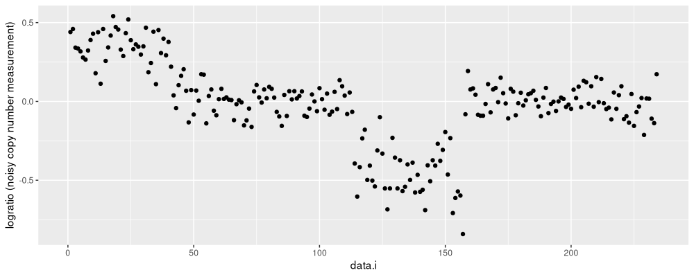
The figure above shows a black dot for each data point to segment.
Binary segmentation
We will consider a parametric model: change in mean with constant variance. Assuming the normal distribution, maximizing the likelihood is equivalent to minimizing the square loss. For an efficient implementation of binary segmentation in this case, we can use the cumulative sum trick.
(cum.dt <- one.dt[, data.table(
  data=c(0,cumsum(logratio)),
  square=c(0,cumsum(logratio^2)))])
##            data     square
##           <num>      <num>
##   1:  0.0000000  0.0000000
##   2:  0.4404207  0.1939704
##   3:  0.8998523  0.4050478
##   4:  1.2412689  0.5216131
##   5:  1.5769808  0.6343156
##  ---
## 231: -4.8383284 16.5655262
## 232: -4.8211191 16.5658223
## 233: -4.9304778 16.5777817
## 234: -5.0681256 16.5967286
## 235: -4.8956381 16.6264805
The output above is a table of cumulative sums of the data and their square.
This table is useful because it allows constant time computation of the optimal square loss for any given segment, for example the segment (1,N) on all of the data:
square_loss <- function(start, end)cum.dt[
, square[end+1]-square[start]-(data[end+1]-data[start])^2/(end+1-start)]
N_data <- nrow(one.dt)
(loss <- square_loss(1, N_data))
## [1] 16.52406
Binary segmentation via splitting
For a segment with N data, we can compute the loss of each candidate split on that segment in linear O(N) time via
get_diff <- function(start, end, change){
  loss_together <- square_loss(start, end)
  loss_apart <- square_loss(start, change)+square_loss(change+1, end)
  data.table(start, end, change, loss_diff=loss_together-loss_apart)
}
get_diff_for_seg <- function(start, end){
  get_diff(start, end, seq(start, end-1L))
}
(first_candidates <- get_diff_for_seg(1, N_data))
##      start   end change    loss_diff
##      <num> <int>  <int>        <num>
##   1:     1   234      1 2.137501e-01
##   2:     1   234      2 4.472175e-01
##   3:     1   234      3 5.741959e-01
##   4:     1   234      4 7.014441e-01
##   5:     1   234      5 8.165622e-01
##  ---
## 229:     1   234    229 8.883904e-04
## 230:     1   234    230 1.769531e-04
## 231:     1   234    231 4.665382e-05
## 232:     1   234    232 2.965470e-03
## 233:     1   234    233 3.756760e-02
Each row in the table above represents a candidate change-point after splitting the first segment (1,N).
The loss_diff column can be maximized to obtain the best split point.
first_candidates[which.max(loss_diff)]
##    start   end change loss_diff
##    <num> <int>  <int>     <num>
## 1:     1   234     41  6.884693
The output above shows that the best first split is a change after data point 41. The code below implements this update rule recursively:
new.segs <- data.table(start=1L, end=N_data)
split.dt.list <- list()
loss <- square_loss(1, N_data)
cand.segs <- NULL
for(n_segs in seq(1, N_data)){
  new.loss <- new.segs[
  , get_diff_for_seg(start, end)[which.max(loss_diff)]
  , by=.I]
  cand.segs <- rbind(cand.segs, new.loss)
  best.i <- which.max(cand.segs$loss_diff)
  best <- cand.segs[best.i]
  split.dt.list[[n_segs]] <- data.table(
    iteration=n_segs,
    segments=n_segs,
    n_in_max=nrow(cand.segs),
    computed=nrow(new.segs),
    best,
    loss)
  loss <- loss-best$loss_diff
  new.segs <- best[, rbind(
    data.table(start, end=change),
    data.table(start=change+1L, end))]
  cand.segs <- cand.segs[-best.i]
}
(split.dt <- rbindlist(split.dt.list))
##      iteration segments n_in_max computed     I start   end change     loss_diff          loss
##          <int>    <int>    <int>    <int> <int> <int> <int>  <int>         <num>         <num>
##   1:         1        1        1        1     1     1   234     41  6.884693e+00  1.652406e+01
##   2:         2        2        2        2     2    42   234    157  1.359552e+00  9.639364e+00
##   3:         3        3        3        2     1    42   157    113  5.763202e+00  8.279812e+00
##   4:         4        4        4        2     2   114   157    152  2.553715e-01  2.516610e+00
##   5:         5        5        5        2     1   114   152    146  1.000791e-01  2.261238e+00
##  ---
## 230:       230      230        4        2     2    64    65     64  4.105069e-06  8.403455e-06
## 231:       231      231        3        2     2    53    54     53  3.283239e-06  4.298387e-06
## 232:       232      232        2        2     2   230   231    230  1.015147e-06  1.015147e-06
## 233:       233      233        1        2     2   164   165    164 -1.734723e-18 -2.955684e-15
## 234:       234      234        0        2    NA    NA    NA     NA            NA -2.953949e-15
plot(loss ~ segments, split.dt)
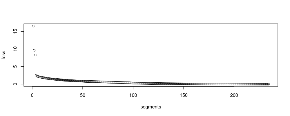
The output table above has one row per split in classic divisive binary segmentation, referred to as Binary segmentation in section 5.2.2 of the Truong review paper.
The figure represents the loss as a function of model size, and is often used for model selection using the slope heuristic (choose the model where the loss starts to become flat).
The R code above is sub-optimal in time and space complexity, because a new cand.segs table must be allocated in each iteration (worst case linear time).
The number of candidates considered changes with the number of segments, as can be seen below.
split.long <- melt(split.dt, measure.vars=c("n_in_max", "computed"))
ggplot()+
  geom_point(aes(
    iteration, value),
    data=split.long)+
  facet_grid(variable ~ ., scales="free")
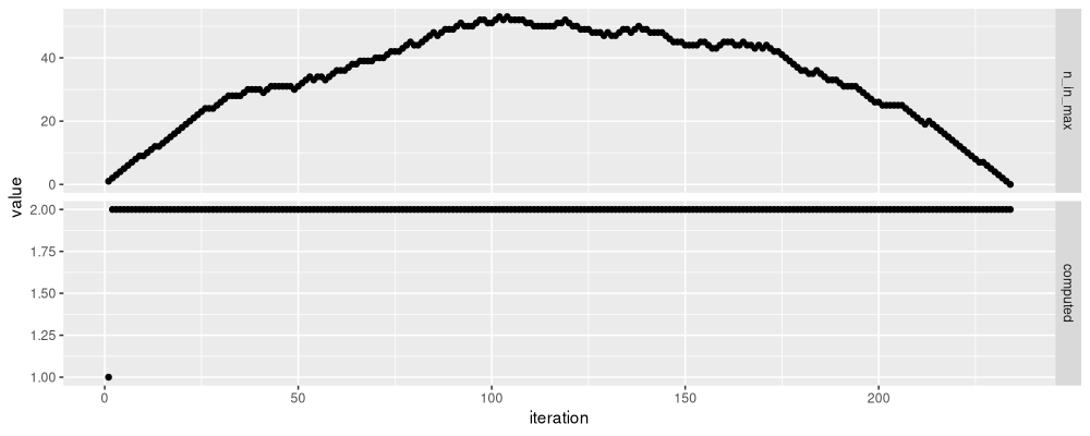
The output above shows that the number of candidates grows to about 50
in the first 100 segments. So the algorithm is quadratic time, and
this could be fixed by moving the code to C++, as in the
binsegRcpp
package, which uses special STL containers (multiset,
priority_queue) to achieve best case log-linear time complexity.
Agglomerative binary segmentation (bottom-up)
Another way to compute change-points is by starting with N separate clusters/segments, and performing N-1 join operations, until we obtain a single cluster/segment. Like the classic divisive binary segmentation described in the previous section, this is a hierarchical segmentation method (result is a tree), and it is referred to as Bottom-up segmentation in section 5.2.3 of the Truong review paper. It is implemented below.
join.dt.list <- list()
join.edge.list <- list()
iteration <- 1
cluster.dt <- data.table(start=1:N_data, end=1:N_data, loss_diff=NA_real_)
while(nrow(cluster.dt)>1){
  todo <- cluster.dt[-.N, which(is.na(loss_diff))]
  new.edges <- cluster.dt[, get_diff(start[todo], end[todo+1], end[todo])]
  cluster.dt[todo, loss_diff := new.edges$loss_diff]
  best.i <- which.min(cluster.dt$loss_diff)
  join.edge.list[[paste(nrow(cluster.dt))]] <- data.table(
    iteration,
    cluster.dt[-.N])[
    , Loss_Difference := ifelse(loss_diff<1e-9, 0, loss_diff)
    ][, let(
      optimal = "no",
      updated = "no"
    )][
      todo, updated := "yes"
    ][
      best.i, optimal := "yes"
    ]
  join.dt.list[[paste(nrow(cluster.dt))]] <- data.table(
    iteration,
    segments=nrow(cluster.dt),
    n_in_min=nrow(cluster.dt),
    computed=length(todo),
    cluster.dt[best.i])
  cluster.dt[best.i-1, loss_diff := NA_real_]
  new.start <- cluster.dt$start[best.i]
  cluster.dt[best.i+1, let(start = new.start, loss_diff = NA_real_)]
  cluster.dt <- cluster.dt[-best.i]
  setkey(cluster.dt, start)
  iteration <- iteration+1L
}
(join.dt <- rbindlist(join.dt.list)[, loss := cumsum(loss_diff)][])
##      iteration segments n_in_min computed start   end     loss_diff          loss
##          <num>    <int>    <int>    <int> <int> <int>         <num>         <num>
##   1:         1      234      234      233   164   164 -1.734723e-18 -1.734723e-18
##   2:         2      233      233        2   230   230  1.015147e-06  1.015147e-06
##   3:         3      232      232        2    53    53  3.283239e-06  4.298387e-06
##   4:         4      231      231        2    64    64  4.105069e-06  8.403455e-06
##   5:         5      230      230        2     3     3  1.627131e-05  2.467477e-05
##  ---
## 229:       229        6        6        2   114   142  7.071936e-02  2.261238e+00
## 230:       230        5        5        2   114   152  2.553715e-01  2.516610e+00
## 231:       231        4        4        2     1    41  3.115634e+00  5.632244e+00
## 232:       232        3        3        1   114   157  5.835662e+00  1.146791e+01
## 233:       233        2        2        1     1   113  5.056151e+00  1.652406e+01
plot(loss ~ segments, join.dt)
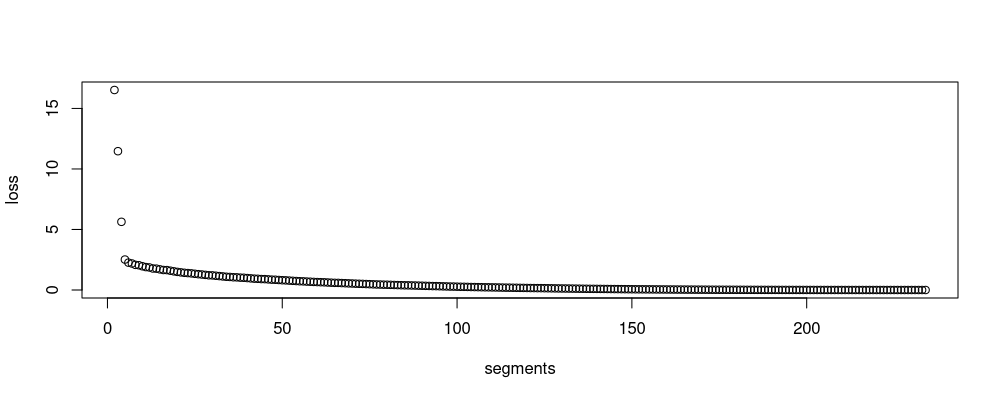
The output above is another table, where the end column represents the sequence of change-points.
The loss figure above is similar to the one in the previous section.
Below we plot the first and last few iterations of the algorithm.
join.edge <- rbindlist(join.edge.list)
join.show <- join.edge[iteration<3 | iteration>230][
, panel := paste("iteration", iteration)]
ggplot()+
  geom_point(aes(
    end+0.5, log10(Loss_Difference), fill=optimal, color=updated),
    shape=21,
    data=join.show)+
  scale_color_manual(values=c(
    yes="black",
    no="white"))+
  geom_point(aes(
    data.i, logratio),
    shape=1,
    data=data.table(one.dt, panel="data"))+
  facet_grid(panel ~ ., scales="free")+
  scale_x_continuous("Index of data or join position in sequence")
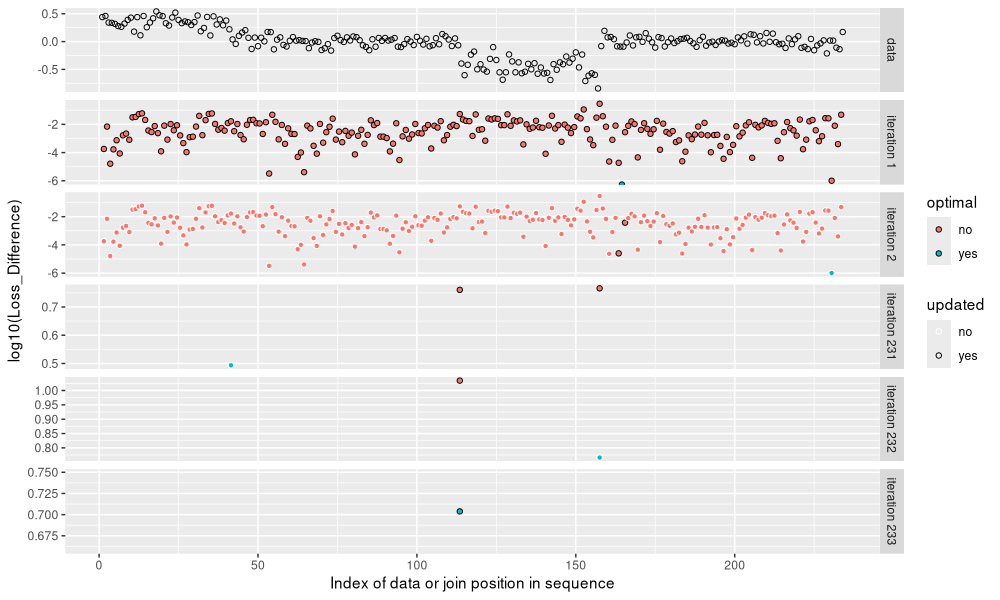
The figure above shows the loss values considered in each iteration of the algorithm, with the data in the top panel as a reference. We can see that the number of candidate loss values starts large, and gradually decreases. Below we plot the number of candidates as a function of number of segments.
join.long <- melt(join.dt, measure.vars=c("n_in_min", "computed"))
ggplot()+
  geom_point(aes(
    iteration, value),
    data=join.long)+
  facet_grid(variable ~ ., scales="free")
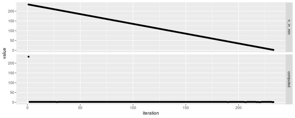
We see a very different pattern in the figure above: the first iteration has the most items in the minimization, which decreases linearly. Using a priority queue in C++ would definitely result in big speed improvements:
- each search for best join would be
O(log N)instead ofO(N), - overall the algorithm would be
O(N log N)instead ofO(N^2).
Comparing the change-points for small model sizes
Do the two algorithms yield the same results? Sometimes, but not always, as we can see in the three examples below.
both.dt <- rbind(
  join.dt[, data.table(algo="join", segments, loss, change=end)],
  split.dt[, data.table(algo="split", segments=segments+1, loss, change)])
show.segs <- 2:4
seg.dt <- data.table(Segments=show.segs)[, {
  both.dt[segments<=Segments, {
    schange <- sort(change)
    start <- c(1L, schange+1L)
    end <- c(schange, N_data)
    total <- cum.dt[, data[end+1]-data[start] ]
    data.table(start, end, mean=total/(end+1-start))
  }, by=algo]
}, by=Segments]
loss.text <- both.dt[segments %in% show.segs][, Segments := segments]
model.color <- "blue"
ggplot()+
  scale_x_continuous(
    limits=c(0, nrow(one.dt)+1))+
  scale_y_continuous(
    "logratio (noisy copy number measurement)")+
  geom_point(aes(
    data.i, logratio),
    data=one.dt)+
  geom_vline(aes(
    xintercept=start-0.5),
    data=seg.dt[start>1],
    linewidth=1,
    linetype="dashed",
    color=model.color)+
  geom_segment(aes(
    start-0.5, mean,
    xend=end+0.5, yend=mean),
    data=seg.dt,
    linewidth=2,
    color=model.color)+
  geom_text(aes(
    230, -0.5, label=sprintf("loss=%.1f", loss)),
    data=loss.text,
    hjust=1,
    color=model.color)+
  facet_grid(Segments ~ algo, labeller=label_both)
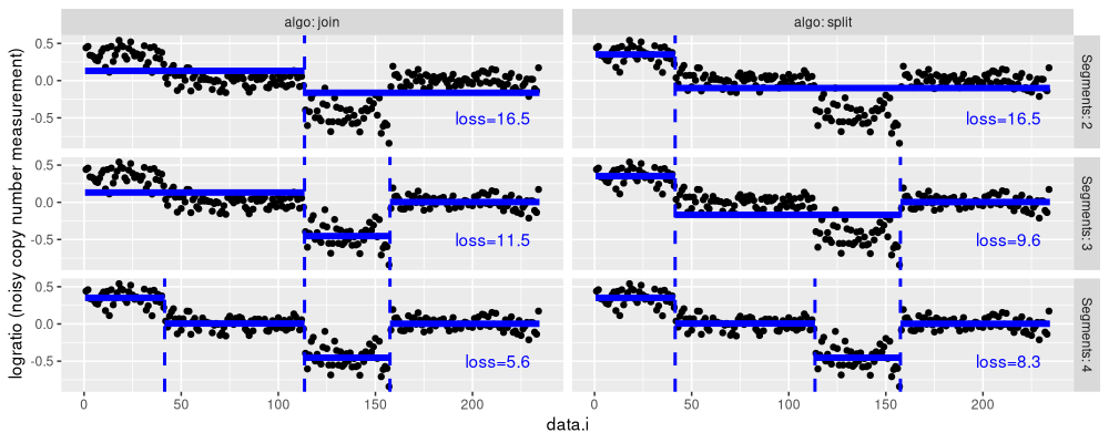
The figure above shows the results for the two algorithms (panels from left to right), and three model sizes (panels from top to bottom).
- For two segments,
algo=splithas a smaller loss value. - For three segments,
algo=joinhas a smaller loss value. - For four segments, both algorithms are the same.
Comparing all loss values
Another way to compare is by examining the loss values for some small model sizes:
show.max <- 19
ggplot()+
  theme_bw()+
  geom_point(aes(
    segments, loss, color=algo, size=algo),
    data=both.dt[segments<=show.max])+
  scale_size_manual(values=c(
    join=3,
    split=2))+
  scale_x_continuous(breaks=1:show.max)
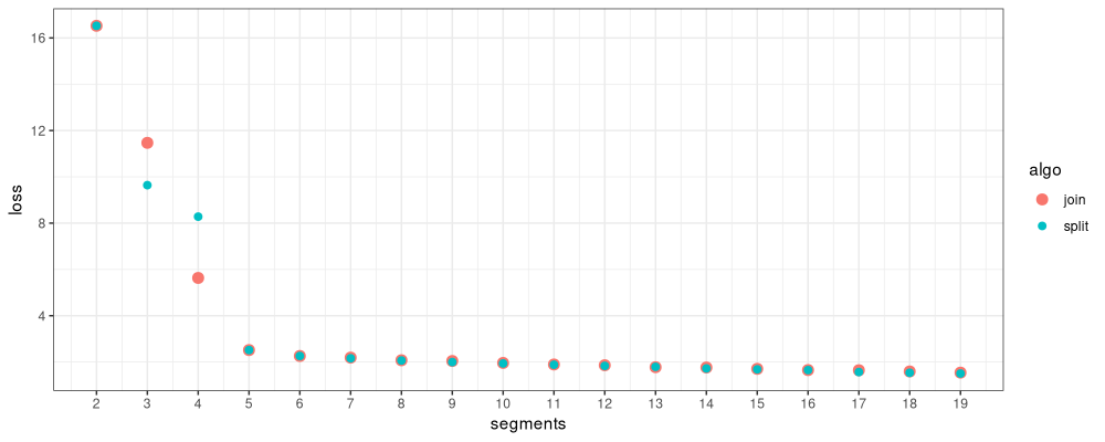
Above we see that there are large loss differences for two small models (2 and 3 segments), and small differences for larger models.
wide.dt <- dcast(both.dt, segments ~ algo, value.var="loss")[
, diff := join-split
][
  !is.na(diff)
][, let(better = fcase(
  abs(diff)<1e-9, "same",
  join<split, "join",
  default="split"
))][]
ggplot()+
  geom_point(aes(
    segments, abs(diff), color=better),
    data=wide.dt)+
  scale_y_log10("Absolute loss difference")+
  scale_color_discrete(breaks=c("split","join","same"))+
  theme(legend.position.inside=c(0.5,0.5))
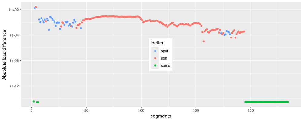
Above we see the absolute loss difference as a function of model size. We see that sometimes the two algorithms result in equally good loss values, and sometimes one is better than the other.
Comparing with hierarchical clustering
Note that the algorithms implemented above are similar to another classic algorithm: agglomerative/hierarchical clustering, implemented as hclust() in R.
But these are not the same in general! See my slides on hierarchical clustering for details about how it works.
Briefly, the hierarchical clustering algorithm starts with N clusters, one for each data point, and computes pairwise distances, represented in an NxN matrix.
It then searches for the min distance, which takes O(N^2) time, and joins the corresponding clusters.
Repeating this join operation N times results in the cluster tree, overall O(N^3) time in general.
There are various ways to speed this up:
- using a priority queue to compute the min distance can reduce an
Nfactor tolog N. - restricting the number of pairwise distances to a neighborhood graph can reduce the
N^2number of distances to minimize over toN(for example on a 2d grid).
Visualizing pairwise distance matrices
Below we code a simple (inefficient) method in R. The first step is to compute the pairwise distance matrix, shown below.
data.mat <- as.matrix(one.dt[, c("logratio")])
data.mat.dt <- data.table(
  row=as.integer(row(data.mat)),
  col=as.integer(col(data.mat)),
  logratio=as.numeric(data.mat))
nb.dist <- dist(data.mat)
nb.dist.mat <- as.matrix(nb.dist)
nb.dist.dt <- data.table(
  iteration=0L,
  row=as.integer(row(nb.dist.mat)),
  col=as.integer(col(nb.dist.mat)),
  dist=as.numeric(nb.dist.mat))
ggplot()+
  geom_tile(aes(
    col, row, fill=dist),
    data=nb.dist.dt)+
  scale_fill_gradient(low="white", high="red")+
  coord_equal()+
  scale_y_reverse("observation")+
  scale_x_continuous("observation")
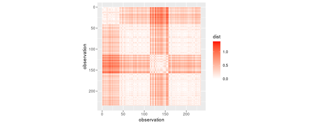
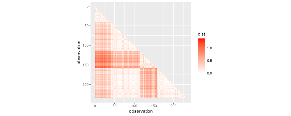
The figure above shows the pairwise distance matrix as a heatmap. Since it is symmetric, we can keep only the lower triangle, without losing information.
lower.triangle <- nb.dist.dt[col<row]
ggplot()+
  geom_tile(aes(
    col, row, fill=dist),
    data=lower.triangle)+
  scale_fill_gradient(low="white", high="red")+
  coord_equal()+
  scale_y_reverse("observation")+
  scale_x_continuous("observation")

The figure above shows the lower triangle, representing distances that we could potentially use in the clustering algorithm. The first iteration of the algorithm uses only the distances in the diagonal band shown below.
diag.band <- nb.dist.dt[col+1==row]
ggplot()+
  geom_tile(aes(
    col, row, fill=dist),
    data=diag.band)+
  scale_fill_gradient(low="white", high="red")+
  coord_equal()+
  scale_y_reverse("observation")+
  scale_x_continuous("observation")
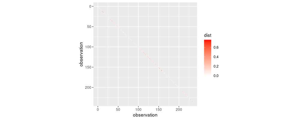
It is difficult to see the band which is one lower than the diagonal in the figure above. Because there is only a diagonal band (1d join constraints), we get a linear time initialization (rather than quadratic as in the usual multivariate clustering algorithm). Are these the same values as in agglomerative binary segmentation?
compare.first.iteration <- data.table(join.edge[iteration==1, .(loss_diff)], diag.band)
ggplot()+
  geom_point(aes(
    loss_diff, dist),
    shape=1,
    data=compare.first.iteration)+
  scale_x_log10()+
  scale_y_log10()
## Warning in transformation$transform(x): Production de NaN
## Warning in scale_x_log10(): log-10 transformation introduced infinite values.
## Warning in scale_y_log10(): log-10 transformation introduced infinite values.
## Warning: Removed 1 row containing missing values or values outside the scale range
## (`geom_point()`).
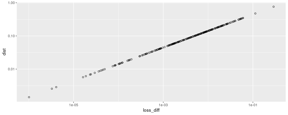
The figure above shows that for the first iteration of this distance/linkage clustering algorithm, the distances on the Y axis are consistent with the loss difference values from the previous loss minimization binary segment joining algorithm.
Clustering algorithm
Below we code the iterations of the clustering algorithm.
Some parts of the code below are similar to the previous algorithm above, but there is a new dist_next column (instead of the previous loss_diff column).
Distance updates use the single linkage criterion: distance between two clusters is defined as the min distance between points in clusters.
agg.dt.list <- list()
agg.edge.list <- list()
iteration <- 1
cluster.dt <- data.table(start=1:N_data, end=1:N_data, dist_next=c(diag.band$dist, NA))
more.dist.list <- list()
more_dist <- function(side, set.i, out.i, in.i){
  out.indices <- with(cluster.dt[out.i], start:end)
  in.indices <- with(cluster.dt[in.i], start:end)
  out.to.in <- nb.dist.mat[out.indices, in.indices, drop=FALSE]
  more.dist.list[[paste(iteration, side)]] <<- data.table(
    iteration,
    CJ(row=out.indices, col=in.indices),
    dist=as.numeric(t(out.to.in)))
  cluster.dt[set.i, dist_next := min(out.to.in, dist_next)]
}
while(nrow(cluster.dt)>1){
  agg.edge.list[[paste(nrow(cluster.dt))]] <- data.table(
    iteration,
    cluster.dt[-.N])
  best.i <- cluster.dt[-.N, which.min(dist_next)]
  agg.dt.list[[paste(nrow(cluster.dt))]] <- data.table(
    iteration,
    segments=nrow(cluster.dt),
    n_in_min=nrow(cluster.dt)-1,
    cluster.dt[best.i])
  if(best.i>1){
    more_dist("before", best.i-1, best.i-1, best.i+1)
  }
  if(best.i+1 < nrow(cluster.dt)){
    more_dist("after", best.i+1, best.i+2, best.i)
  }
  new.start <- cluster.dt$start[best.i]
  cluster.dt[best.i+1, start := new.start]
  cluster.dt <- cluster.dt[-best.i]
  iteration <- iteration+1L
}
(agg.dt <- rbindlist(agg.dt.list))
##      iteration segments n_in_min start   end   dist_next
##          <num>    <int>    <num> <int> <int>       <num>
##   1:         1      234      233   164   164 0.000000000
##   2:         2      233      232   230   230 0.001424884
##   3:         3      232      231    53    53 0.002562514
##   4:         4      231      230    64    64 0.002865334
##   5:         5      230      229     3     3 0.005704614
##  ---
## 229:       229        6        5   115   115 0.006562688
## 230:       230        5        4   114   114 0.005676185
## 231:       231        4        3     1   113 0.001545469
## 232:       232        3        2     1   156 0.133266531
## 233:       233        2        1     1   157 0.000000000
The result table above shows one row per iteration of the clustering algorithm. Below we compare with iterations of the previous algorithm.
(agg.changes <- data.table(agg.dt[, .(
  iteration, segments, distance=end
)], loss=join.dt$end))
##      iteration segments distance  loss
##          <num>    <int>    <int> <int>
##   1:         1      234      164   164
##   2:         2      233      230   230
##   3:         3      232       53    53
##   4:         4      231       64    64
##   5:         5      230        3     3
##  ---
## 229:       229        6      115   142
## 230:       230        5      114   152
## 231:       231        4      113    41
## 232:       232        3      156   157
## 233:       233        2      157   113
Above we see a table with one row per iteration of the clustering algorithm. The first few rows show that the same join events are chosen for the first few iterations, but in general they are not the same. And in fact the last iterations of the algorithm are quite different.
show.segs <- 2:4
agg.seg.dt <- data.table(Segments=show.segs)[, {
  data.table(minimize=c("distance","loss"))[, {
    change <- agg.changes[segments<=Segments][[minimize]]
    schange <- sort(change)
    start <- c(1L, schange+1L)
    end <- c(schange, N_data)
    total <- cum.dt[, data[end+1]-data[start] ]
    data.table(
      start,
      end,
      mean=total/(end+1-start),
      square_loss=square_loss(start, end))
  }, by=minimize]
}, by=Segments]
agg.loss.dt <- agg.seg.dt[, .(
  loss=sum(square_loss)
), by=.(minimize, Segments)]
model.color <- "blue"
ggplot()+
  scale_x_continuous(
    limits=c(0, nrow(one.dt)+1))+
  scale_y_continuous(
    "logratio (noisy copy number measurement)")+
  geom_point(aes(
    data.i, logratio),
    data=one.dt)+
  geom_vline(aes(
    xintercept=start-0.5),
    data=agg.seg.dt[start>1],
    linewidth=1,
    linetype="dashed",
    color=model.color)+
  geom_segment(aes(
    start-0.5, mean,
    xend=end+0.5, yend=mean),
    data=agg.seg.dt,
    linewidth=2,
    color=model.color)+
  geom_text(aes(
    230, -0.5, label=sprintf("loss=%.3f", loss)),
    data=agg.loss.dt,
    hjust=1,
    color=model.color)+
  facet_grid(Segments ~ minimize, labeller=label_both)
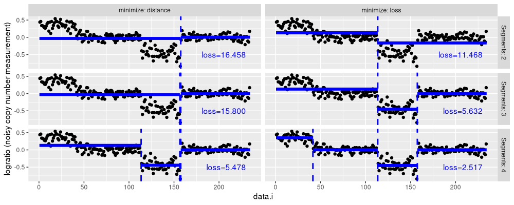
The figure above shows several agglomerative clustering models, using either distance or loss minimization. We see that in general they are quite different (min/single linkage used, so Ward linkage should give different results). Below we visualize the distances computed by the algorithm.
more.dist <- rbindlist(more.dist.list)
used.dist <- rbind(diag.band, more.dist)[, let(
  pmin = pmin(row,col),
  pmax = pmax(row,col))][]
ggplot()+
  geom_tile(aes(
    pmin, pmax, fill=dist),
    data=used.dist)+
  scale_fill_gradient(low="white", high="red")+
  coord_equal()+
  scale_y_reverse("observation")+
  scale_x_continuous("observation")
It can be seen that all of the lower triangle was used in the single linkage clustering algorithm. It is substantially less efficient than the loss-based binary segmentation, which would be log-linear with an efficient C++ implementation. Below we visualize the number of distance matrix entries computed in each iteration.
count.dist <- used.dist[, .(computed=.N), by=iteration]
plot(log10(computed) ~ iteration, count.dist)
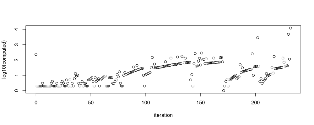
Above we see the number of distances increases with the number of iterations.
Conclusions
We have explored different methods for segmentation of data in 1d, using either loss minimization segmentation (divisive or bottom up joining), or distance minimization clustering (joining).
Session info
sessionInfo()
## R Under development (unstable) (2025-05-21 r88220)
## Platform: x86_64-pc-linux-gnu
## Running under: Ubuntu 24.04.3 LTS
##
## Matrix products: default
## BLAS:   /usr/lib/x86_64-linux-gnu/blas/libblas.so.3.12.0
## LAPACK: /usr/lib/x86_64-linux-gnu/lapack/liblapack.so.3.12.0  LAPACK version 3.12.0
##
## locale:
##  [1] LC_CTYPE=fr_FR.UTF-8       LC_NUMERIC=C               LC_TIME=fr_FR.UTF-8        LC_COLLATE=fr_FR.UTF-8     LC_MONETARY=fr_FR.UTF-8
##  [6] LC_MESSAGES=fr_FR.UTF-8    LC_PAPER=fr_FR.UTF-8       LC_NAME=C                  LC_ADDRESS=C               LC_TELEPHONE=C
## [11] LC_MEASUREMENT=fr_FR.UTF-8 LC_IDENTIFICATION=C
##
## time zone: America/Toronto
## tzcode source: system (glibc)
##
## attached base packages:
## [1] stats     graphics  grDevices utils     datasets  methods   base
##
## other attached packages:
## [1] ggplot2_3.5.2      data.table_1.17.99
##
## loaded via a namespace (and not attached):
##  [1] labeling_0.4.3     RColorBrewer_1.1-3 R6_2.6.1           tidyselect_1.2.1   xfun_0.53          farver_2.1.2       magrittr_2.0.4
##  [8] gtable_0.3.6       glue_1.8.0         tibble_3.3.0       knitr_1.50         pkgconfig_2.0.3    generics_0.1.4     dplyr_1.1.4
## [15] lifecycle_1.0.4    cli_3.6.5          scales_1.4.0       grid_4.6.0         vctrs_0.6.5        withr_3.0.2        compiler_4.6.0
## [22] tools_4.6.0        pillar_1.11.0      evaluate_1.0.5     rlang_1.1.6