Bike ride map and time series data viz
The goal of this post is to explain how to use animint2, my R package for animated interactive data visualization, to create a linked map and time series of bike rides I did in 2009.
Background: master internship motivation for interactive graphics
Since my master internship at INRA Jouy-en-Josas in 2009, I had some ideas about using interactive data visualization to better understand complex data and algorithms. At that time, I was studying an iterative sampling algorithm for inferring the parameters of a hierarchical Bayesian model. The best visualization tools at the time were lattice/ggplot2 and animation packages in R. Using that approach, the only interactions possible are moving forward and backward in time, which resulted in data visualizations such as this one, which remarkably still works after 15 years! You can click play and watch the animation like a video, but clicking on the plots does not accomplish any interaction.
But it could be useful to be able to click the plot, for example to update the selected locus or time point! That is called “direct manipulation” in the interactive graphics literature. How could I make graphics with those kinds of interactions? They are a very specific kind of interaction, “click on some visual element, to change the highlighted value of some variable.” (locus or generation in that example) At the end of my master internship, I decided to shift gears, and focus on studying the math behind machine learning, so these interactive graphics ideas sat on the backburner of my mind for a few years.
First version of animint
In 2012, I defended my PHD in Paris, and then flew out to Tokyo to spend 2013 in Masashi Sugiyama’s machine learning lab. During that time, I got to working on my interactive graphics ideas again, this time with a focus on visualizing machine learning algorithms. I coded a first version of the animint R package, and Susan VanderPlas worked in GSOC’13 to implement a bunch of key features. I then created a first gallery of examples, including a re-make of my master internship data viz, but with the interactive features that I had envisioned. On that web page,
- the left plot shows a time series for the selected locus, and you can click to select a different time point (generation).
- the right plot shows an overview of all loci for the selected time point (generation), and you can click to select a different locus.
How do we define that data visualization? We use R/ggplot2 code, with two new keywords that can be defined for any geom:
showSelectedmeans to only show data rows that correspond to the values of the current selection.clickSelectsmeans that the geom can be clicked to change the current selection.
The code on that web page uses the old animint package, which is no longer recommended. Below we port the code to the new animint2 package, which is recommended:
library(animint2)
data(generation.loci)
##generation.loci <- subset(generation.loci, generation %% 10 == 1)
colormap <- c(blue="blue",red="red",ancestral="black",neutral="grey30")
ancestral <- subset(generation.loci,population==1 & generation==1)
ancestral$color <- "ancestral"
viz <- animint(
  title="Evolution simulation with drift and selection",
  source="https://tdhock.github.io/blog/2025/bike-ride-data-viz/",
  ts=ggplot()+
    ggtitle("Click to select generation")+
    theme(legend.position="none")+
    geom_line(aes(
      generation, frequency, group=paste(population,color),
      colour=color),
      showSelected=c("locus","color"),
      data=generation.loci)+
    make_text(generation.loci, 50, 1.05, "locus")+
    make_tallrect(generation.loci, "generation")+
    scale_colour_manual("population", values=colormap)+
    geom_point(aes(
      generation, frequency, color=color),
      showSelected=c("locus","color"),
      data=ancestral),
  loci=ggplot()+
    ggtitle("Click to select locus")+
    geom_point(aes(
      locus, frequency, colour=color,
      key=paste(locus, population)),
      showSelected="generation",
      chunk_vars=character(),
      data=generation.loci)+
    geom_point(aes(
      locus, frequency, colour=color),
      data=ancestral)+
    scale_colour_manual("population", values=colormap)+
    make_tallrect(generation.loci, "locus")+
    make_text(generation.loci, 35, 1, "generation"),
  duration=list(generation=1000),
  time=list(variable="generation", ms=2000))
if(FALSE){
  animint2pages(viz, "2025-01-19-evolution-drift-selection")
}
The interactive data viz created using the code above can be viewed here. Using this method, it is remarkably simple to create a wide variety of different data visualizations. The point of the original gallery was to highlight the variety of different kinds of visualizations which are possible to create. The modern gallery contains a much larger array of example data visualizations, but remarkably does not contain the interaction instructions that were present in the original gallery (click X to change Y). That kind of information can be very useful for somebody who does not know how to interact with the data visualization. Similar “help the user understand what interactions are possible” features are planned for the upcoming GSOC’25, which will hopefully implement a guided tour and tutorial videos.
Back to the master
Right now I am working in Paris again, and I thought it would be fun to re-visit another old project, gpsdb, GPS data website generator. For my birthday in 2009, my classmates gifted me a GPS, which I used to create data sets for my bike rides in and around Paris. The gpsdb software was a couple of python scripts that could download data from the GPS, and then convert it to KML files, which were required for visualizing the data on google maps, back in the day. Remarkably, the web site that I created, and those data files, are still online, 15 years later. For example all.kml contains all of the GPS traces I created in 2009. However google maps no longer accepts arbitrary KML files (these are too large), so how can we visualize them? Below we explain how to do it using animint2.
Clone gpsdb and read GPS data
First step: clone the repository to get the GPS data.
if(!file.exists("gpsdb-code")){
  system("hg clone http://hg.code.sf.net/p/gpsdb/code gpsdb-code")
}
gpx.glob <- "gpsdb-code/gpx/*"
library(data.table)
(gpx.dt <- data.table(gpx=Sys.glob(gpx.glob)))
##                                         gpx
##                                      <char>
##   1: gpsdb-code/gpx/2009-04-09:18:11:56.gpx
##   2: gpsdb-code/gpx/2009-04-11:09:52:48.gpx
##   3: gpsdb-code/gpx/2009-04-11:15:51:05.gpx
##   4: gpsdb-code/gpx/2009-04-13:11:59:58.gpx
##   5: gpsdb-code/gpx/2009-04-13:16:39:34.gpx
##  ---
## 114: gpsdb-code/gpx/2009-10-07:18:41:11.gpx
## 115: gpsdb-code/gpx/2009-10-11:08:51:39.gpx
## 116: gpsdb-code/gpx/2009-10-11:12:10:11.gpx
## 117: gpsdb-code/gpx/2009-10-25:07:22:37.gpx
## 118: gpsdb-code/gpx/2009-10-25:10:25:19.gpx
The table above shows one row for each GPX data file. Each one of them has contents as below:
one.file <- gpx.dt$gpx[1]
gpx.lines <- readLines(one.file)
cat(gpx.lines[1:20],sep="\n")
## <?xml version="1.0" encoding="UTF-8"?>
## <gpx
## version="1.0"
## xmlns:xsi="http://www.w3.org/2001/XMLSchema-instance"
## xmlns="http://www.topografix.com/GPX/1/0"
## xsi:schemaLocation="http://www.topografix.com/GPX/1/0 http://www.topografix.com/GPX/1/0/gpx.xsd">
## <trk>
## <name>/home/thocking/kml/2009-04-09:18:11:56</name>
## <trkseg>
## <trkpt lat="2.17865" lon="48.76205">
## 	<ele>0.0</ele>
## </trkpt>
## <trkpt lat="2.17978" lon="48.76171">
## 	<ele>0.0</ele>
## </trkpt>
## <trkpt lat="2.18143" lon="48.76177">
## 	<ele>0.0</ele>
## </trkpt>
## <trkpt lat="2.18326" lon="48.76138">
## 	<ele>0.0</ele>
The output above includes lat and lon values that we would like to extract and visualize on a map. But oddly, these files have lat and lon reversed (Paris is actually near longitude=2 degrees, not latitude=2 degrees as is shown in the output above). To read these data, we can use the function below, which switches lat and lon:
name_pat <- function(name, pattern)list(
  pattern, '="',
  nc::group(name, "[0-9.]+", as.numeric))
read_lat_lon <- function(path)nc::capture_all_str(
  path,
  name_pat("longitude","lat"),
  '" ',
  name_pat("latitude","lon"))
read_lat_lon(one.file)
##      longitude latitude
##          <num>    <num>
##   1:   2.17865 48.76205
##   2:   2.17978 48.76171
##   3:   2.18143 48.76177
##   4:   2.18326 48.76138
##   5:   2.18473 48.76063
##  ---
## 194:   2.33935 48.81965
## 195:   2.33933 48.81964
## 196:   2.33931 48.81964
## 197:   2.33932 48.81966
## 198:   2.33932 48.81966
The code above uses regular expressions to read the GPS data. The
name_pat function is useful for defining a pattern that occurs twice
(lat and lon). The read_lat_lon function returns a data table with
longitude and latitude columns, and one row for each GPS ping in
the file, as can be seen in the output above.
To read all of the files into a data table, we use the code below,
(lat.lon.dt <- nc::capture_first_glob(
  gpx.glob,
  "/", timestamp="[^/]+", "[.]gpx$",
  READ=read_lat_lon))
##                  timestamp longitude latitude
##                     <char>     <num>    <num>
##     1: 2009-04-09:18:11:56   2.17865 48.76205
##     2: 2009-04-09:18:11:56   2.17978 48.76171
##     3: 2009-04-09:18:11:56   2.18143 48.76177
##     4: 2009-04-09:18:11:56   2.18326 48.76138
##     5: 2009-04-09:18:11:56   2.18473 48.76063
##    ---
## 23832: 2009-10-25:10:25:19   2.36657 48.86880
## 23833: 2009-10-25:10:25:19   2.36660 48.86878
## 23834: 2009-10-25:10:25:19   2.36663 48.86874
## 23835: 2009-10-25:10:25:19   2.36666 48.86870
## 23836: 2009-10-25:10:25:19   2.36666 48.86870
The output above includes a timestamp column which comes from the
file name, and the other columns which come from the result of reading
the file contents. The gpx.glob defines a set of file names, which
are matched to the provided pattern, with named arguments/groups
included in the output (timestamp). The READ argument specifies
how to read each file, via the read_lat_lon function.
Already we can visualize these data on a map:
library(animint2)
ggplot()+
  geom_path(aes(
    longitude, latitude, group=timestamp),
    data=lat.lon.dt)
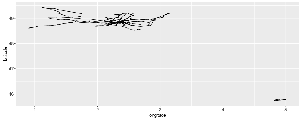
In the plot above, we see that there is a large set of data in the upper left, and a small amount of data in the lower right. We can zoom to the upper left via the code below:
path.show <- lat.lon.dt[longitude < 4]
(gg.path <- ggplot()+
  geom_path(aes(
    longitude, latitude, group=timestamp),
    data=path.show))
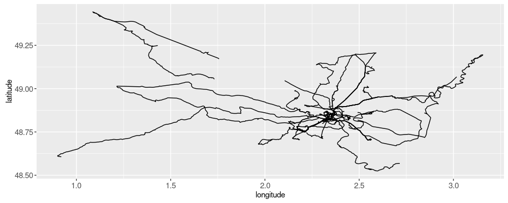
The figure above kind of looks like a spider web, with the center being Paris.
We can add details about the start and end of each trip via the code below:
start.end.dt <- path.show[
, .SD[c(1,.N), .(
  latitude,longitude,where=c("start","end"),
  direction=diff(longitude))]
, by=timestamp]
gg.path+
  geom_point(aes(
    longitude, latitude, fill=where),
    shape=21,
    data=start.end.dt)+
  scale_fill_manual(values=c(start="white",end="black"))
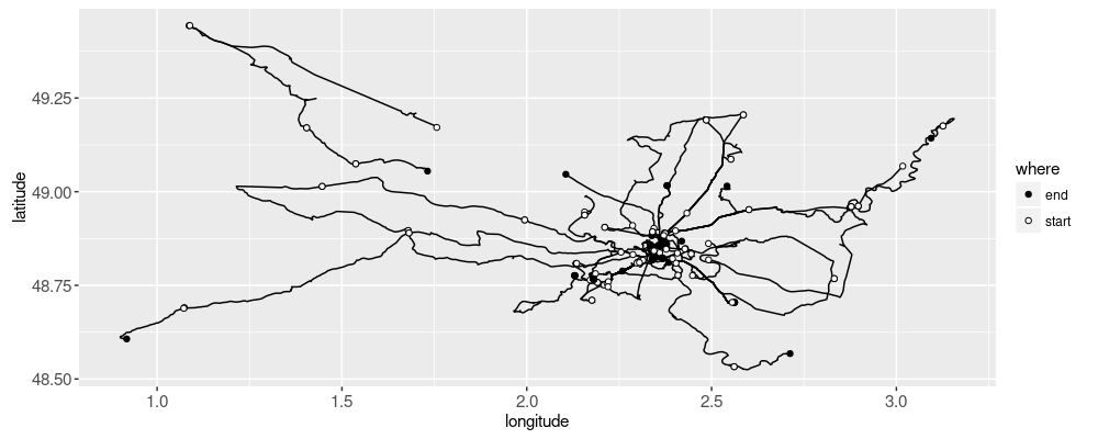
The plot above shows a dot at the start and end of each trip.
Context: nearby cities
The current map is not super useful currently, because we do not see names of the start/end cities (nor a familiar unit of distance like kilometers). To get the context of nearby cities, we can download a data set which has lat/lon coordinates of each city in France.
if(!file.exists("gps-villes-de-france.csv")){
  download.file("https://www.data.gouv.fr/fr/datasets/r/51606633-fb13-4820-b795-9a2a575a72f1", "gps-villes-de-france.csv")
}
(villes.dt <- fread("gps-villes-de-france.csv"))
##        insee_code           city_code zip_code               label  latitude   longitude    department_name
##            <char>              <char>    <int>              <char>     <num>       <num>             <char>
##     1:      25620       ville du pont    25650       ville du pont  46.99987    6.498147              doubs
##     2:      25624      villers grelot    25640      villers grelot  47.36151    6.235167              doubs
##     3:      25615 villars les blamont    25310 villars les blamont  47.36838    6.871415              doubs
##     4:      25619       les villedieu    25240       les villedieu  46.71391    6.265831              doubs
##     5:      25622       villers buzon    25170       villers buzon  47.22856    5.852187              doubs
##    ---
## 39141:      98829                thio    98829                thio        NA          NA nouvelle-calédonie
## 39142:      98831                 voh    98833                 voh        NA          NA nouvelle-calédonie
## 39143:      98832                yate    98834                yate        NA          NA nouvelle-calédonie
## 39144:      98612              sigave    98620              sigave -14.27041 -178.155263   wallis-et-futuna
## 39145:      98613                uvea    98600                uvea -13.28186 -176.161928   wallis-et-futuna
##        department_number             region_name     region_geojson_name
##                   <char>                  <char>                  <char>
##     1:                25 bourgogne-franche-comté Bourgogne-Franche-Comté
##     2:                25 bourgogne-franche-comté Bourgogne-Franche-Comté
##     3:                25 bourgogne-franche-comté Bourgogne-Franche-Comté
##     4:                25 bourgogne-franche-comté Bourgogne-Franche-Comté
##     5:                25 bourgogne-franche-comté Bourgogne-Franche-Comté
##    ---
## 39141:               988      nouvelle-calédonie      Nouvelle Calédonie
## 39142:               988      nouvelle-calédonie      Nouvelle Calédonie
## 39143:               988      nouvelle-calédonie      Nouvelle Calédonie
## 39144:               986        wallis-et-futuna        Wallis-et-Futuna
## 39145:               986        wallis-et-futuna        Wallis-et-Futuna
ggplot()+
  geom_point(aes(
    longitude, latitude),
    data=villes.dt)
## Warning: Removed 211 rows containing missing values (geom_point).
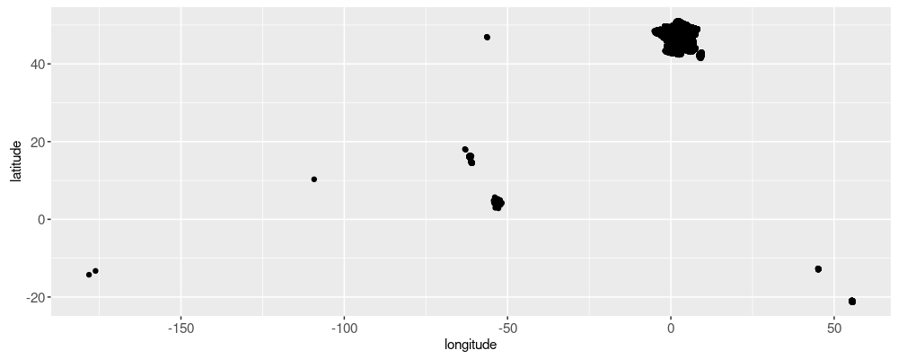
Looking at the plot above, we see a hexagon in the upper right, which
corresponds to “France métropolitaine” (mainland European France). The
other points correspond to outlying islands and other territories. Our
map only needs context of the Paris region, so we don’t want to
display all of these cities. Let’s just display the nearest cities to
the start and end. To do that we can use
sf::st_nearest_feature,
but first we have to convert our data to sf structures, as in the
code below.
sf::st_pointcreates a single geometry representing a point on a map.sf::st_sfccreates a list column of geometries,sf::st_sfcreates a data frame with a simple feature list column (so you can associate various other data to each geometry, such as timestamp, etc).
(start.end.sf <- sf::st_sf(start.end.dt[, .(
  timestamp, where,
  geometry=sf::st_sfc(apply(
    cbind(longitude, latitude),
    1,
    sf::st_point,
    simplify=FALSE
  ))
)]))
## Simple feature collection with 228 features and 2 fields
## Geometry type: POINT
## Dimension:     XY
## Bounding box:  xmin: 0.91765 ymin: 48.53294 xmax: 3.1262 ymax: 49.44358
## CRS:           NA
## First 10 features:
##              timestamp where                 geometry
## 1  2009-04-09:18:11:56 start POINT (2.17865 48.76205)
## 2  2009-04-09:18:11:56   end POINT (2.33932 48.81966)
## 3  2009-04-11:09:52:48 start POINT (2.44841 48.77634)
## 4  2009-04-11:09:52:48   end POINT (2.56225 48.70457)
## 5  2009-04-11:15:51:05 start POINT (2.56225 48.70456)
## 6  2009-04-11:15:51:05   end POINT (2.33981 48.82073)
## 7  2009-04-13:11:59:58 start POINT (2.35749 48.85656)
## 8  2009-04-13:11:59:58   end POINT (2.36255 48.87485)
## 9  2009-04-13:16:39:34 start  POINT (2.3549 48.84662)
## 10 2009-04-13:16:39:34   end POINT (2.33974 48.82025)
(villes.sf <- sf::st_sf(villes.dt[, .(
  label,
  geometry=sf::st_sfc(apply(
    cbind(longitude, latitude),
    1,
    sf::st_point,
    simplify=FALSE
  ))
)]))
## Simple feature collection with 39145 features and 1 field (with 211 geometries empty)
## Geometry type: POINT
## Dimension:     XY
## Bounding box:  xmin: -178.1553 ymin: -21.33962 xmax: 55.75454 ymax: 51.07291
## CRS:           NA
## First 10 features:
##                     label                  geometry
## 1           ville du pont POINT (6.498147 46.99987)
## 2          villers grelot POINT (6.235167 47.36151)
## 3     villars les blamont POINT (6.871415 47.36838)
## 4           les villedieu POINT (6.265831 46.71391)
## 5           villers buzon POINT (5.852187 47.22856)
## 6        villers la combe POINT (6.473842 47.24081)
## 7  villers sous chalamont POINT (6.045328 46.90159)
## 8            voujeaucourt POINT (6.782506 47.47355)
## 9    bouconville vauclair POINT (3.756685 49.46019)
## 10             bouresches POINT (3.316703 49.06706)
nearest.index.vec <- sf::st_nearest_feature(start.end.sf, villes.sf)
(villes.start.end <- data.table(
  start.end.dt[,.(timestamp,direction,where)],
  villes.dt[nearest.index.vec]))
##                timestamp direction  where insee_code          city_code zip_code              label latitude longitude
##                   <char>     <num> <char>     <char>             <char>    <int>             <char>    <num>     <num>
##   1: 2009-04-09:18:11:56   0.16067  start      78322      jouy en josas    78350      jouy en josas 48.76589  2.163600
##   2: 2009-04-09:18:11:56   0.16067    end      94037           gentilly    94250           gentilly 48.81327  2.344191
##   3: 2009-04-11:09:52:48   0.11384  start      94028            creteil    94000            creteil 48.78377  2.454729
##   4: 2009-04-11:09:52:48   0.11384    end      94056            perigny    94520 perigny sur yerres 48.69659  2.561137
##   5: 2009-04-11:15:51:05  -0.22244  start      94056            perigny    94520 perigny sur yerres 48.69659  2.561137
##  ---
## 224: 2009-10-11:12:10:11   0.15125    end      77269             maincy    77950             maincy 48.55379  2.706115
## 225: 2009-10-25:07:22:37   0.38605  start      94068 st maur des fosses    94210 st maur des fosses 48.79882  2.494497
## 226: 2009-10-25:07:22:37   0.38605    end      77143    cregy les meaux    77124    cregy les meaux 48.97774  2.873223
## 227: 2009-10-25:10:25:19  -0.51125  start      77143    cregy les meaux    77124    cregy les meaux 48.97774  2.873223
## 228: 2009-10-25:10:25:19  -0.51125    end      75103           paris 03    75003              paris 48.86288  2.359999
##      department_name department_number   region_name region_geojson_name
##               <char>            <char>        <char>              <char>
##   1:        yvelines                78 île-de-france       Île-de-France
##   2:    val-de-marne                94 île-de-france       Île-de-France
##   3:    val-de-marne                94 île-de-france       Île-de-France
##   4:    val-de-marne                94 île-de-france       Île-de-France
##   5:    val-de-marne                94 île-de-france       Île-de-France
##  ---
## 224:  seine-et-marne                77 île-de-france       Île-de-France
## 225:    val-de-marne                94 île-de-france       Île-de-France
## 226:  seine-et-marne                77 île-de-france       Île-de-France
## 227:  seine-et-marne                77 île-de-france       Île-de-France
## 228:           paris                75 île-de-france       Île-de-France
The table above contains one row for each start/end position, and columns that describe the closest nearby city, which can be displayed via:
ggplot()+
  geom_path(aes(
    longitude, latitude, group=timestamp, color=what),
    data=data.table(path.show, what="ride"))+
  geom_point(aes(
    longitude, latitude, fill=where, color=what),
    shape=21,
    data=data.table(start.end.dt, what="ride"))+
  scale_fill_manual(values=c(start="white",end="black"))+
  scale_color_manual(values=c(
    ride="black",
    "nearby cities"="red"))+
  geom_point(aes(
    longitude, latitude, fill=where,
    color=what),
    shape=21,
    data=data.table(villes.start.end, what="nearby cities"))+
  geom_text(aes(
    longitude, latitude, label=label,
    color=what,
    hjust=ifelse(
      direction<0,
      ifelse(where=="start", 0, 1),
      ifelse(where=="start", 1, 0))),
    showSelected=c("timestamp","where"),
    data=data.table(villes.start.end, what="nearby cities"))
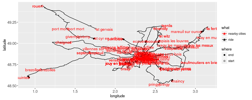
The map above is overplotted, so interactivity is useful to focus on some details. We would like to be able to click on one trip, and show its details only. How to implement that? Using animint2 we would specify
clickSelects="timestamp"to specify that we want to click on an element to specify the selected ride (file timestamp).showSelected="timestamp"to specify that we want to display only the subset of data for the currently selected ride (file timestamp).
The end result looks like this. Exercise for the reader: starting from the code above, can you create the interactive map and time series yourself?
Conclusions
We have explored how to read GPS bike ride data into R, along with
city locations for context, and then display them together on a
map. We explained various features of animint2 for interactive data
visualization, and sf for spatial data manipulation (finding the
closest city to the start/end coordinates of each ride).
Session info
sessionInfo()
## R Under development (unstable) (2024-10-01 r87205)
## Platform: x86_64-pc-linux-gnu
## Running under: Ubuntu 22.04.5 LTS
##
## Matrix products: default
## BLAS:   /usr/lib/x86_64-linux-gnu/blas/libblas.so.3.10.0
## LAPACK: /usr/lib/x86_64-linux-gnu/lapack/liblapack.so.3.10.0
##
## locale:
##  [1] LC_CTYPE=fr_FR.UTF-8       LC_NUMERIC=C               LC_TIME=fr_FR.UTF-8        LC_COLLATE=fr_FR.UTF-8
##  [5] LC_MONETARY=fr_FR.UTF-8    LC_MESSAGES=fr_FR.UTF-8    LC_PAPER=fr_FR.UTF-8       LC_NAME=C
##  [9] LC_ADDRESS=C               LC_TELEPHONE=C             LC_MEASUREMENT=fr_FR.UTF-8 LC_IDENTIFICATION=C
##
## time zone: Europe/Paris
## tzcode source: system (glibc)
##
## attached base packages:
## [1] stats     graphics  utils     datasets  grDevices methods   base
##
## other attached packages:
## [1] animint2_2024.11.27 data.table_1.16.4
##
## loaded via a namespace (and not attached):
##  [1] vctrs_0.6.5        cli_3.6.2          knitr_1.47         rlang_1.1.3        xfun_0.45          highr_0.11
##  [7] DBI_1.2.1          KernSmooth_2.23-24 generics_0.1.3     sf_1.0-15          RJSONIO_1.3-1.9    glue_1.7.0
## [13] labeling_0.4.3     nc_2024.12.17      colorspace_2.1-0   plyr_1.8.9         e1071_1.7-14       fansi_1.0.6
## [19] scales_1.3.0       grid_4.5.0         evaluate_0.23      tibble_3.2.1       munsell_0.5.0      classInt_0.4-10
## [25] lifecycle_1.0.4    compiler_4.5.0     dplyr_1.1.4        pkgconfig_2.0.3    Rcpp_1.0.12        farver_2.1.1
## [31] digest_0.6.34      R6_2.5.1           tidyselect_1.2.1   utf8_1.2.4         class_7.3-22       pillar_1.9.0
## [37] magrittr_2.0.3     tools_4.5.0        proxy_0.4-27       gtable_0.3.4       units_0.8-5