Comparing change-point pruning methods using square loss
The goal of this post is to compare two pruning methods for speeding up the optimal partitioning algorithm, similar to my previous post using the Poisson loss.
- We assume that we want to find change-points in a sequence of
Ndata. - All algorithms discussed are instances of dynamic programming, which
has a for loop over all
Ndata. In each iteration, the algorithm considers a certain number of candidate change-pointsC(on average). The algorithm is overallO(NC)time. - Optimal partitioning (OPART) computes the best segmentation for a
given loss function, data sequence, and non-negative penalty
value. Each iteration considers the loss for each previous candidate
change-point,
C=O(N)linear time per iteration, which implies quadraticO(N^2)time overall. - Pruned Exact Linear Time (PELT) reduces the number of candidate
change-points that must be considered at each iteration, from the
whole data sequence size
N, to the size of a segmentS, soC=O(S). This gives an algorithm which isO(NS)time overall.- If the number of change-points grows linearly with the data size
N, then the segment size is constant,S=O(1)with respect to number of dataN, and the PELT algorithm is indeed linear time overall,O(N). - However in the case of a constant number of change-points, with
segment sizes that grow with the data sequence,
S=O(N)implies quadratic time overall,O(N^2).
- If the number of change-points grows linearly with the data size
- Functional Pruning Optimal Partitioning (FPOP) reduces the number of
candidate change-points to a number which is always less than the
number considered by PELT (see Maidstone 2017 paper for detailed
proof). The goal of this post is to show that it prunes more than
PELT in both cases:
- If the number of change-points grows linearly with the data size
N, then both PELT and FPOP areO(N)overall. - If the number of change-points is constant with respect to data
size
N, then FPOP considers onlyS=O(log N)change-points (empirically), which gives an algorithm that isO(N log N), log-linear time overall.
- If the number of change-points grows linearly with the data size
Simulate data sequences
We simulate data in two scenarios: linear and constant number of changes.
mean_vec <- c(10,20,5,25)
sim_fun_list <- list(
  constant_changes=function(N){
    rep(mean_vec, each=N/4)
  },
  linear_changes=function(N){
    rep(rep(mean_vec, each=10), l=N)
  })
lapply(sim_fun_list, function(f)f(40))
## $constant_changes
##  [1] 10 10 10 10 10 10 10 10 10 10 20 20 20 20 20 20 20 20 20 20  5  5  5  5  5  5  5  5  5  5 25 25 25 25 25 25 25 25
## [39] 25 25
##
## $linear_changes
##  [1] 10 10 10 10 10 10 10 10 10 10 20 20 20 20 20 20 20 20 20 20  5  5  5  5  5  5  5  5  5  5 25 25 25 25 25 25 25 25
## [39] 25 25
As can be seen above, both functions return a vector of values that represent the true segment mean. Below we use both functions with a three different data sizes.
library(data.table)
N_data_vec <- c(40, 400)
sim_data_list <- list()
sim_changes_list <- list()
sim_segs_list <- list()
for(N_data in N_data_vec){
  for(simulation in names(sim_fun_list)){
    sim_fun <- sim_fun_list[[simulation]]
    data_mean_vec <- sim_fun(N_data)
    end <- which(diff(data_mean_vec) != 0)
    set.seed(1)
    data_value <- rnorm(N_data, data_mean_vec, 2)
    cum.vec <- c(0, cumsum(data_value))
    n.segs <- sum(diff(data_mean_vec)!=0)+1
    wfit <- fpopw::Fpsn(data_value, n.segs)
    end <- wfit$t.est[n.segs, 1:n.segs]
    start <- c(1, end[-length(end)]+1)
    sim_segs_list[[paste(N_data, simulation)]] <- data.table(
      N_data, simulation, start.pos=start-0.5, end.pos=end+0.5,
      mean=(cum.vec[end+1]-cum.vec[start])/(end-start+1))
    sim_data_list[[paste(N_data, simulation)]] <- data.table(
      N_data, simulation, data_i=seq_along(data_value), data_value)
    sim_changes_list[[paste(N_data, simulation)]] <- data.table(
      N_data, simulation, end)
  }
}
addSim <- function(DT)DT[, Simulation := paste0("\n", simulation)][]
(sim_changes <- addSim(rbindlist(sim_changes_list)))
##     N_data       simulation   end         Simulation
##      <num>           <char> <num>             <char>
##  1:     40 constant_changes    10 \nconstant_changes
##  2:     40 constant_changes    20 \nconstant_changes
##  3:     40 constant_changes    30 \nconstant_changes
##  4:     40 constant_changes    40 \nconstant_changes
##  5:     40   linear_changes    10   \nlinear_changes
##  6:     40   linear_changes    20   \nlinear_changes
##  7:     40   linear_changes    30   \nlinear_changes
##  8:     40   linear_changes    40   \nlinear_changes
##  9:    400 constant_changes   100 \nconstant_changes
## 10:    400 constant_changes   200 \nconstant_changes
## 11:    400 constant_changes   300 \nconstant_changes
## 12:    400 constant_changes   400 \nconstant_changes
## 13:    400   linear_changes    10   \nlinear_changes
## 14:    400   linear_changes    20   \nlinear_changes
## 15:    400   linear_changes    30   \nlinear_changes
## 16:    400   linear_changes    40   \nlinear_changes
## 17:    400   linear_changes    50   \nlinear_changes
## 18:    400   linear_changes    60   \nlinear_changes
## 19:    400   linear_changes    70   \nlinear_changes
## 20:    400   linear_changes    80   \nlinear_changes
## 21:    400   linear_changes    90   \nlinear_changes
## 22:    400   linear_changes   100   \nlinear_changes
## 23:    400   linear_changes   110   \nlinear_changes
## 24:    400   linear_changes   120   \nlinear_changes
## 25:    400   linear_changes   130   \nlinear_changes
## 26:    400   linear_changes   140   \nlinear_changes
## 27:    400   linear_changes   150   \nlinear_changes
## 28:    400   linear_changes   160   \nlinear_changes
## 29:    400   linear_changes   170   \nlinear_changes
## 30:    400   linear_changes   180   \nlinear_changes
## 31:    400   linear_changes   190   \nlinear_changes
## 32:    400   linear_changes   200   \nlinear_changes
## 33:    400   linear_changes   210   \nlinear_changes
## 34:    400   linear_changes   220   \nlinear_changes
## 35:    400   linear_changes   230   \nlinear_changes
## 36:    400   linear_changes   240   \nlinear_changes
## 37:    400   linear_changes   250   \nlinear_changes
## 38:    400   linear_changes   260   \nlinear_changes
## 39:    400   linear_changes   270   \nlinear_changes
## 40:    400   linear_changes   280   \nlinear_changes
## 41:    400   linear_changes   290   \nlinear_changes
## 42:    400   linear_changes   300   \nlinear_changes
## 43:    400   linear_changes   310   \nlinear_changes
## 44:    400   linear_changes   320   \nlinear_changes
## 45:    400   linear_changes   330   \nlinear_changes
## 46:    400   linear_changes   340   \nlinear_changes
## 47:    400   linear_changes   350   \nlinear_changes
## 48:    400   linear_changes   360   \nlinear_changes
## 49:    400   linear_changes   370   \nlinear_changes
## 50:    400   linear_changes   380   \nlinear_changes
## 51:    400   linear_changes   390   \nlinear_changes
## 52:    400   linear_changes   400   \nlinear_changes
##     N_data       simulation   end         Simulation
##      <num>           <char> <num>             <char>
Above we see the table of simulated change-points.
Below we visualize one of the simulated data sets.
library(ggplot2)
one_sim <- sim_data_list[["40 constant_changes"]]
gg <- ggplot()+
  theme_bw()+
  theme(text=element_text(size=14))+
  geom_point(aes(
    data_i, data_value),
    color="grey50",
    data=one_sim)+
  scale_x_continuous(
    breaks=seq(0,max(N_data_vec),by=10))
gg
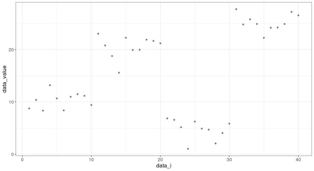
The figure above shows a simulated data set with 40 points.
wfit <- fpopw::Fpop(one_sim$data_value, 50)
cum.vec <- c(0, cumsum(one_sim$data_value))
end <- wfit$t.est
start <- c(1, end[-length(end)]+1)
one_sim_means <- data.table(
  start.pos=start-0.5, end.pos=end+0.5,
  mean=(cum.vec[end+1]-cum.vec[start])/(end-start+1))
gg+
  geom_vline(aes(
    xintercept=start.pos),
    color="green",
    linetype="dashed",
    data=one_sim_means[-1])+
  geom_segment(aes(
    start.pos, mean,
    xend=end.pos, yend=mean),
    color="green",
    data=one_sim_means)
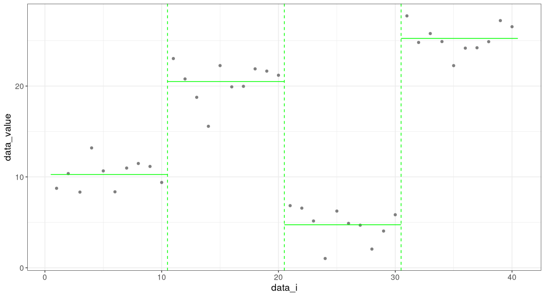
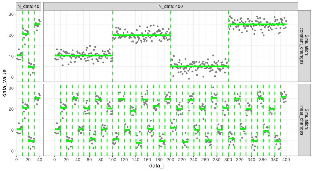
Below we show all simulations:
- For
constant_changessimulation, there are always 3 change-points. - For
linear_changessimulation, there are more change-points when there are more data.
(sim_data <- addSim(rbindlist(sim_data_list)))
##      N_data       simulation data_i data_value         Simulation
##       <num>           <char>  <int>      <num>             <char>
##   1:     40 constant_changes      1   8.747092 \nconstant_changes
##   2:     40 constant_changes      2  10.367287 \nconstant_changes
##   3:     40 constant_changes      3   8.328743 \nconstant_changes
##   4:     40 constant_changes      4  13.190562 \nconstant_changes
##   5:     40 constant_changes      5  10.659016 \nconstant_changes
##  ---
## 876:    400   linear_changes    396  23.151374   \nlinear_changes
## 877:    400   linear_changes    397  28.185828   \nlinear_changes
## 878:    400   linear_changes    398  25.090021   \nlinear_changes
## 879:    400   linear_changes    399  23.569743   \nlinear_changes
## 880:    400   linear_changes    400  26.730446   \nlinear_changes
library(ggplot2)
gg <- ggplot()+
  theme_bw()+
  theme(text=element_text(size=14))+
  geom_point(aes(
    data_i, data_value),
    color="grey50",
    data=sim_data)+
  facet_grid(Simulation ~ N_data, labeller=label_both, scales="free_x", space="free")+
  scale_x_continuous(
    breaks=seq(0,max(N_data_vec),by=20))
gg
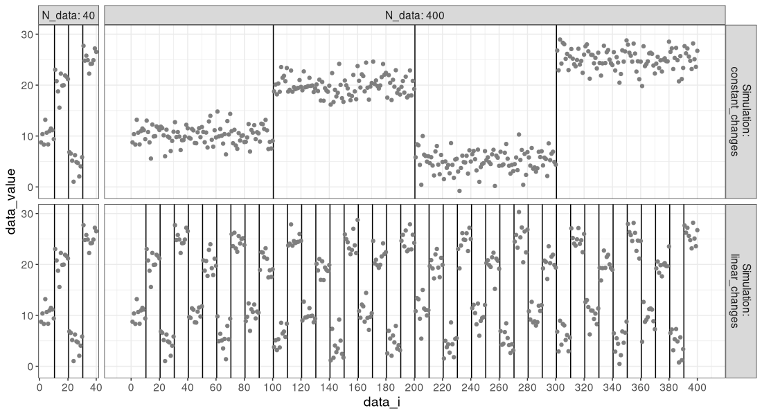
We see in the figure above that the data are the same in the two simulations, when there are only 40 data points. However, when there are 80 or 160 data, we see a difference:
- For the
constant_changessimulation, the number of change-points is still three (change-point every quarter of the data). - For the
linear_changessimulation, the number of change-points has increased from 3 to 7 to 15 (change-point every 25 data points).
Below we highlight the true change-points,
gg+
  geom_vline(aes(
    xintercept=end+0.5),
    data=sim_changes)
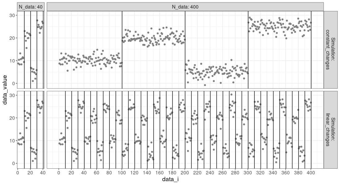
And below we show the estimated means and change-points:
sim_segs <- addSim(rbindlist(sim_segs_list))
gg+
  geom_vline(aes(
    xintercept=start.pos),
    color="green",
    linetype="dashed",
    size=1,
    data=sim_segs[1<start.pos])+
  geom_segment(aes(
    start.pos, mean,
    xend=end.pos, yend=mean),
    data=sim_segs,
    color="green",
    size=2)
## Warning: Using `size` aesthetic for lines was deprecated in ggplot2 3.4.0.
## ℹ Please use `linewidth` instead.
## This warning is displayed once every 8 hours.
## Call `lifecycle::last_lifecycle_warnings()` to see where this warning was generated.
PELT
Below we define a function which implements PELT for the Poisson loss, because we used a count data simulation above.
PELT <- function(sim.mat, penalty, prune=TRUE, verbose=FALSE){
  if(!is.matrix(sim.mat))sim.mat <- cbind(sim.mat)
  cum.data <- rbind(0, apply(sim.mat, 2, cumsum))
  sum_trick <- function(m, start, end)m[end+1,,drop=FALSE]-m[start,,drop=FALSE]
  cost_trick <- function(start, end){
    sum_vec <- sum_trick(cum.data, start, end)
    N <- end+1-start
    -sum_vec^2/N
  }
  N.data <- nrow(sim.mat)
  pelt.change.vec <- rep(NA_integer_, N.data)
  pelt.cost.vec <- rep(NA_real_, N.data+1)
  pelt.cost.vec[1] <- -penalty
  pelt.candidates.vec <- rep(NA_integer_, N.data)
  candidate.vec <- 1L
  if(verbose)index_dt_list <- list()
  for(up.to in 1:N.data){
    N.cand <- length(candidate.vec)
    pelt.candidates.vec[up.to] <- N.cand
    last.seg.cost <- rowSums(cost_trick(candidate.vec, rep(up.to, N.cand)))
    prev.cost <- pelt.cost.vec[candidate.vec]
    cost.no.penalty <- prev.cost+last.seg.cost
    total.cost <- cost.no.penalty+penalty
    if(verbose)index_dt_list[[up.to]] <- data.table(
      data_i=up.to, change_i=candidate.vec, cost=total.cost/up.to)
    best.i <- which.min(total.cost)
    pelt.change.vec[up.to] <- candidate.vec[best.i]
    total.cost.best <- total.cost[best.i]
    pelt.cost.vec[up.to+1] <- total.cost.best
    keep <- if(isTRUE(prune))cost.no.penalty < total.cost.best else TRUE
    candidate.vec <- c(candidate.vec[keep], up.to+1L)
  }
  list(
    change=pelt.change.vec,
    cost=pelt.cost.vec,
    candidates=pelt.candidates.vec,
    index_dt=if(verbose)rbindlist(index_dt_list))
}
decode <- function(best.change){
  seg.dt.list <- list()
  last.i <- length(best.change)
  while(last.i>0){
    first.i <- best.change[last.i]
    seg.dt.list[[paste(last.i)]] <- data.table(
      first.i, last.i)
    last.i <- first.i-1L
  }
  rbindlist(seg.dt.list)[seq(.N,1)]
}
pelt_info_list <- list()
pelt_segs_list <- list()
both_index_list <- list()
penalty <- 100
algo.prune <- c(
  OPART=FALSE,
  PELT=TRUE)
for(N_data in N_data_vec){
  for(simulation in names(sim_fun_list)){
    N_sim <- paste(N_data, simulation)
    data_value <- sim_data_list[[N_sim]]$data_value
    for(algo in names(algo.prune)){
      prune <- algo.prune[[algo]]
      fit <- PELT(data_value, penalty=penalty, prune=prune, verbose = TRUE)
      both_index_list[[paste(N_data, simulation, algo)]] <- data.table(
        N_data, simulation, algo, fit$index_dt)
      fit_seg_dt <- decode(fit$change)
      pelt_info_list[[paste(N_data,simulation,algo)]] <- data.table(
        N_data,simulation,algo,
        candidates=fit$candidates,
        cost=fit$cost[-1],
        data_i=seq_along(data_value))
      pelt_segs_list[[paste(N_data,simulation,algo)]] <- data.table(
        N_data,simulation,algo,
        fit_seg_dt)
    }
  }
}
(pelt_info <- addSim(rbindlist(pelt_info_list)))
##       N_data       simulation   algo candidates          cost data_i         Simulation
##        <num>           <char> <char>      <int>         <num>  <int>             <char>
##    1:     40 constant_changes  OPART          1     -76.51163      1 \nconstant_changes
##    2:     40 constant_changes  OPART          2    -182.67974      2 \nconstant_changes
##    3:     40 constant_changes  OPART          3    -251.04164      3 \nconstant_changes
##    4:     40 constant_changes  OPART          4    -412.77406      4 \nconstant_changes
##    5:     40 constant_changes  OPART          5    -526.18819      5 \nconstant_changes
##   ---
## 1756:    400   linear_changes   PELT          6 -109335.43620    396   \nlinear_changes
## 1757:    400   linear_changes   PELT          7 -110124.86554    397   \nlinear_changes
## 1758:    400   linear_changes   PELT          8 -110753.45859    398   \nlinear_changes
## 1759:    400   linear_changes   PELT          9 -111303.80462    399   \nlinear_changes
## 1760:    400   linear_changes   PELT         10 -112017.39690    400   \nlinear_changes
(pelt_segs <- addSim(rbindlist(pelt_segs_list)))
##      N_data       simulation   algo first.i last.i         Simulation
##       <num>           <char> <char>   <int>  <int>             <char>
##   1:     40 constant_changes  OPART       1     10 \nconstant_changes
##   2:     40 constant_changes  OPART      11     20 \nconstant_changes
##   3:     40 constant_changes  OPART      21     30 \nconstant_changes
##   4:     40 constant_changes  OPART      31     40 \nconstant_changes
##   5:     40 constant_changes   PELT       1     10 \nconstant_changes
##  ---
## 100:    400   linear_changes   PELT     351    360   \nlinear_changes
## 101:    400   linear_changes   PELT     361    370   \nlinear_changes
## 102:    400   linear_changes   PELT     371    380   \nlinear_changes
## 103:    400   linear_changes   PELT     381    390   \nlinear_changes
## 104:    400   linear_changes   PELT     391    400   \nlinear_changes
We see in the result tables above that the segmentations are the same, using pruning and no pruning. Below we visualize the number of candidates considered.
algo.colors <- c(
  OPART="grey50",
  PELT="red",
  FPOP="blue",
  DUST="deepskyblue")
cat(paste0("\\definecolor{", names(algo.colors), "}{HTML}{", sub("#", "", animint2::toRGB(algo.colors)), "}\n"))
## Registered S3 methods overwritten by 'animint2':
##   method                   from
##   [.uneval                 ggplot2
##   drawDetails.zeroGrob     ggplot2
##   grid.draw.absoluteGrob   ggplot2
##   grobHeight.absoluteGrob  ggplot2
##   grobHeight.zeroGrob      ggplot2
##   grobWidth.absoluteGrob   ggplot2
##   grobWidth.zeroGrob       ggplot2
##   grobX.absoluteGrob       ggplot2
##   grobY.absoluteGrob       ggplot2
##   heightDetails.titleGrob  ggplot2
##   heightDetails.zeroGrob   ggplot2
##   makeContext.dotstackGrob ggplot2
##   print.element            ggplot2
##   print.ggplot2_bins       ggplot2
##   print.rel                ggplot2
##   print.theme              ggplot2
##   print.uneval             ggplot2
##   widthDetails.titleGrob   ggplot2
##   widthDetails.zeroGrob    ggplot2
## \definecolor{OPART}{HTML}{7F7F7F}
##  \definecolor{PELT}{HTML}{FF0000}
##  \definecolor{FPOP}{HTML}{0000FF}
##  \definecolor{DUST}{HTML}{00BFFF}
ggplot()+
  theme_bw()+
  theme(
    legend.position=c(0.8, 0.2),
    panel.spacing=grid::unit(1,"lines"),
    text=element_text(size=15))+
  geom_vline(aes(
    xintercept=end+0.5),
    data=sim_changes)+
  scale_color_manual(
    breaks=names(algo.colors),
    values=algo.colors)+
  geom_point(aes(
    data_i, candidates, color=algo),
    data=pelt_info)+
  facet_grid(Simulation ~ N_data, labeller=label_both, scales="free_x", space="free")+
  scale_x_continuous(
    breaks=seq(0,max(N_data_vec),by=20))+
  scale_y_continuous(
    breaks=c(10, 100, 400))+
  theme(panel.grid.minor=element_blank())+
  coord_cartesian(expand=FALSE)
## Warning: A numeric `legend.position` argument in `theme()` was deprecated in ggplot2 3.5.0.
## ℹ Please use the `legend.position.inside` argument of `theme()` instead.
## This warning is displayed once every 8 hours.
## Call `lifecycle::last_lifecycle_warnings()` to see where this warning was generated.
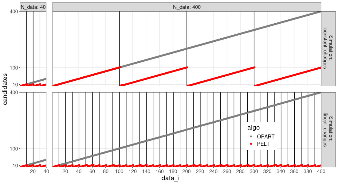
We can see in the figure above that PELT considers a much smaller number of change-points, that tends to reset near zero, for each change-point detected.
- In the bottom simulation with linear changes, the number of change-point candidates considered by PELT is constant (does not depend on number of data), so PELT is linear time, whereas OPART is quadratic, in the number of data.
- In the top simulation with constant changes, the number of change-point candidates considered by PELT is linear in the number of data, so both OPART and PELT are quadratic time in the number of data.
FPOP
Now we run FPOP, which is another pruning method, which is more complex to implement efficiently, so we use C++ code in the R package fpopw. In fact, the current CRAN version of fpopw (1.1) does not include the code which is used to write the candidate change-points considered at each iteration of dynamic programming, so we need to install my version from GitHub.
remotes::install_github("tdhock/fpopw/fpopw")
## Using github PAT from envvar GITHUB_PAT. Use `gitcreds::gitcreds_set()` and unset GITHUB_PAT in .Renviron (or elsewhere) if you want to use the more secure git credential store instead.
## Downloading GitHub repo tdhock/fpopw@HEAD
## ── R CMD build ─────────────────────────────────────────────────────────────────────────────────────────────────
##
   checking for file ‘/tmp/Rtmp3bxDpD/remotes1832b711e8f3a8/tdhock-fpopw-9d8c9a9/fpopw/DESCRIPTION’ ...

✔  checking for file ‘/tmp/Rtmp3bxDpD/remotes1832b711e8f3a8/tdhock-fpopw-9d8c9a9/fpopw/DESCRIPTION’
##

─  preparing ‘fpopw’:
##    checking DESCRIPTION meta-information ...

✔  checking DESCRIPTION meta-information
## ─  cleaning src
##

─  checking for LF line-endings in source and make files and shell scripts
##

─  checking for empty or unneeded directories
##

─  building ‘fpopw_1.2.tar.gz’
##

   Avis : valeur uid incorrecte remplacée par celle pour l'utilisateur 'nobody'
##    Avis : valeur gid incorrecte remplacée par celle pour l'utilisateur 'nobody'
##


##
fpop_info_list <- list()
fpop_segs_list <- list()
for(N_data in N_data_vec){
  for(simulation in names(sim_fun_list)){
    N_sim <- paste(N_data, simulation)
    data_value <- sim_data_list[[N_sim]]$data_value
    pfit <- fpopw::Fpop(
      data_value, penalty, verbose_file=tempfile())
    both_index_list[[paste(N_data, simulation, "FPOP")]] <- data.table(
      N_data, simulation, algo="FPOP", pfit$model
    )[, let(
      data_i=data_i+1L,
      change_i=ifelse(change_i == -10, 0, change_i)+1
    )][]
    end <- pfit$t.est
    start <- c(1, end[-length(end)]+1)
    count_dt <- pfit$model[, .(
      intervals=.N,
      cost=min(cost)
    ), by=data_i]
    fpop_info_list[[paste(N_data,simulation)]] <- data.table(
      N_data,simulation,
      algo="FPOP",
      candidates=count_dt$intervals,
      cost=count_dt$cost,
      data_i=seq_along(data_value))
    fpop_segs_list[[paste(N_data,simulation)]] <- data.table(
      N_data,simulation,start,end)
  }
}
(fpop_info <- addSim(rbindlist(fpop_info_list)))
##      N_data       simulation   algo candidates         cost data_i         Simulation
##       <num>           <char> <char>      <int>        <num>  <int>             <char>
##   1:     40 constant_changes   FPOP          1     -76.5116      1 \nconstant_changes
##   2:     40 constant_changes   FPOP          2    -182.6800      2 \nconstant_changes
##   3:     40 constant_changes   FPOP          3    -251.0420      3 \nconstant_changes
##   4:     40 constant_changes   FPOP          3    -412.7740      4 \nconstant_changes
##   5:     40 constant_changes   FPOP          4    -526.1880      5 \nconstant_changes
##  ---
## 876:    400   linear_changes   FPOP          2 -109335.0000    396   \nlinear_changes
## 877:    400   linear_changes   FPOP          4 -110125.0000    397   \nlinear_changes
## 878:    400   linear_changes   FPOP          3 -110753.0000    398   \nlinear_changes
## 879:    400   linear_changes   FPOP          3 -111304.0000    399   \nlinear_changes
## 880:    400   linear_changes   FPOP          4 -112017.0000    400   \nlinear_changes
(fpop_segs <- rbindlist(fpop_segs_list))
##     N_data       simulation start   end
##      <num>           <char> <num> <int>
##  1:     40 constant_changes     1    10
##  2:     40 constant_changes    11    20
##  3:     40 constant_changes    21    30
##  4:     40 constant_changes    31    40
##  5:     40   linear_changes     1    10
##  6:     40   linear_changes    11    20
##  7:     40   linear_changes    21    30
##  8:     40   linear_changes    31    40
##  9:    400 constant_changes     1   100
## 10:    400 constant_changes   101   200
## 11:    400 constant_changes   201   300
## 12:    400 constant_changes   301   400
## 13:    400   linear_changes     1    10
## 14:    400   linear_changes    11    20
## 15:    400   linear_changes    21    30
## 16:    400   linear_changes    31    40
## 17:    400   linear_changes    41    50
## 18:    400   linear_changes    51    60
## 19:    400   linear_changes    61    70
## 20:    400   linear_changes    71    80
## 21:    400   linear_changes    81    90
## 22:    400   linear_changes    91   100
## 23:    400   linear_changes   101   110
## 24:    400   linear_changes   111   120
## 25:    400   linear_changes   121   130
## 26:    400   linear_changes   131   140
## 27:    400   linear_changes   141   150
## 28:    400   linear_changes   151   160
## 29:    400   linear_changes   161   170
## 30:    400   linear_changes   171   180
## 31:    400   linear_changes   181   190
## 32:    400   linear_changes   191   200
## 33:    400   linear_changes   201   210
## 34:    400   linear_changes   211   220
## 35:    400   linear_changes   221   230
## 36:    400   linear_changes   231   240
## 37:    400   linear_changes   241   250
## 38:    400   linear_changes   251   260
## 39:    400   linear_changes   261   270
## 40:    400   linear_changes   271   280
## 41:    400   linear_changes   281   290
## 42:    400   linear_changes   291   300
## 43:    400   linear_changes   301   310
## 44:    400   linear_changes   311   320
## 45:    400   linear_changes   321   330
## 46:    400   linear_changes   331   340
## 47:    400   linear_changes   341   350
## 48:    400   linear_changes   351   360
## 49:    400   linear_changes   361   370
## 50:    400   linear_changes   371   380
## 51:    400   linear_changes   381   390
## 52:    400   linear_changes   391   400
##     N_data       simulation start   end
##      <num>           <char> <num> <int>
both_info <- rbind(pelt_info, fpop_info)
ggplot()+
  theme_bw()+
  theme(
    legend.position=c(0.8, 0.2),
    panel.spacing=grid::unit(1,"lines"),
    text=element_text(size=15))+
  geom_vline(aes(
    xintercept=end+0.5),
    data=sim_changes)+
  scale_color_manual(
    breaks=names(algo.colors),
    values=algo.colors)+
  geom_point(aes(
    data_i, candidates, color=algo),
    data=both_info)+
  facet_grid(Simulation ~ N_data, labeller=label_both, scales="free_x", space="free")+
  scale_x_continuous(
    breaks=seq(0,max(N_data_vec),by=20))+
  scale_y_continuous(
    breaks=c(10, 100, 400))+
  theme(panel.grid.minor=element_blank())+
  coord_cartesian(expand=FALSE)
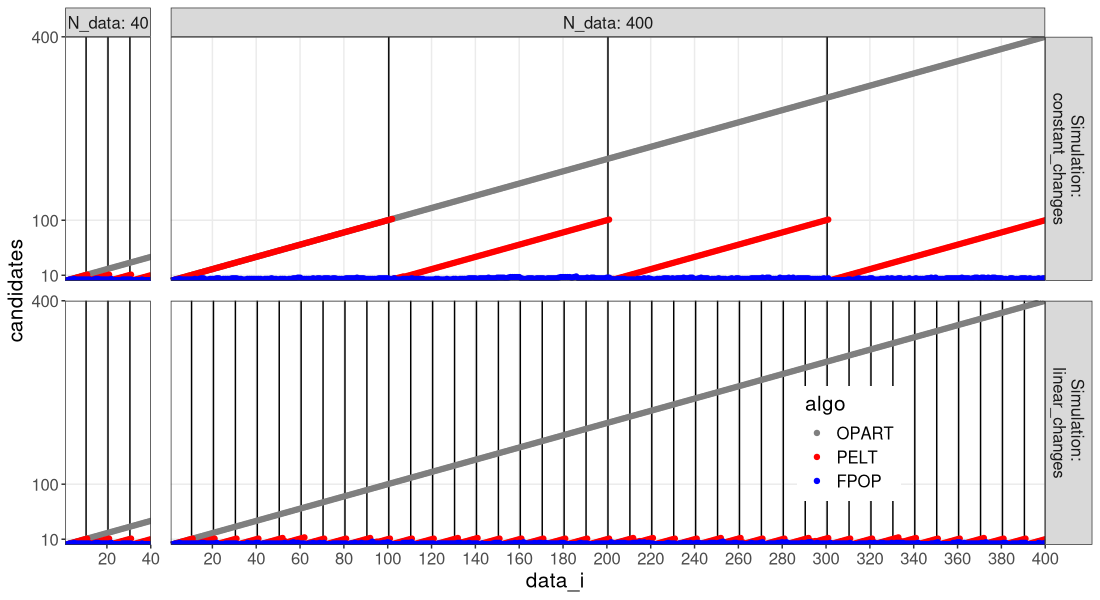
In the figure above, we can see the advantage of FPOP: the number of change-points considered does not increase with the number of data, even with constant number of changes (larger segments).
- In the top simulation with constant changes, the number of change-points candidates considered is linear in the number of data, so both OPART and PELT are quadratic time in the number of data, whereas FPOP is sub-quadratic (empirically linear or log-linear).
The table below compares the cost and number of candidates for the last data point.
both_info[data_i==max(data_i)][order(simulation, algo)]
##    N_data       simulation   algo candidates      cost data_i         Simulation
##     <num>           <char> <char>      <int>     <num>  <int>             <char>
## 1:    400 constant_changes   FPOP          5 -115415.0    400 \nconstant_changes
## 2:    400 constant_changes  OPART        400 -115415.2    400 \nconstant_changes
## 3:    400 constant_changes   PELT        100 -115415.2    400 \nconstant_changes
## 4:    400   linear_changes   FPOP          4 -112017.0    400   \nlinear_changes
## 5:    400   linear_changes  OPART        400 -112017.4    400   \nlinear_changes
## 6:    400   linear_changes   PELT         10 -112017.4    400   \nlinear_changes
We see above that in both simulations, all three algos compute the same cost. We also see that the number of candidates is smallest for FPOP in both simulations. PELT has substantial pruning (10 candidates) for the case of linear changes, but not much pruning (100 candidates) for the case of constant changes.
DuST
DuST is a new pruning technique based on Lagrange duality, proposed by Truong and Runge, Stat, 2024.
remotes::install_github("vrunge/dust@910f8c67f99354fdb5ff7740e6436eb487d9efa6")
## Using github PAT from envvar GITHUB_PAT. Use `gitcreds::gitcreds_set()` and unset GITHUB_PAT in .Renviron (or elsewhere) if you want to use the more secure git credential store instead.
## Downloading GitHub repo vrunge/dust@910f8c67f99354fdb5ff7740e6436eb487d9efa6
## These packages have more recent versions available.
## It is recommended to update all of them.
## Which would you like to update?
##
## 1: All
## 2: CRAN packages only
## 3: None
## 4: RcppArmad... (14.4.1-1 -> 14.4.3-1) [CRAN]
##
## ── R CMD build ─────────────────────────────────────────────────────────────────────────────────────────────────
##
   checking for file ‘/tmp/Rtmp3bxDpD/remotes1832b7352b6c2c/vrunge-dust-910f8c6/DESCRIPTION’ ...

✔  checking for file ‘/tmp/Rtmp3bxDpD/remotes1832b7352b6c2c/vrunge-dust-910f8c6/DESCRIPTION’
##

─  preparing ‘dust’:
##    checking DESCRIPTION meta-information ...

✔  checking DESCRIPTION meta-information
## ─  cleaning src
##

─  checking for LF line-endings in source and make files and shell scripts
##

─  checking for empty or unneeded directories
##

   Omitted ‘LazyData’ from DESCRIPTION
##

─  building ‘dust_0.3.0.tar.gz’
##

   Avis : valeur uid incorrecte remplacée par celle pour l'utilisateur 'nobody'
##    Avis : valeur gid incorrecte remplacée par celle pour l'utilisateur 'nobody'
##


##
set.seed(1)
ex_data <- rnorm(7)
ex_penalty <- 1
dfit <- dust::dust.1D(ex_data, ex_penalty)
wfit <- fpopw::Fpop(ex_data, ex_penalty)
pfit <- PELT(ex_data, ex_penalty)
list(PELT=pfit$change, FPOP=wfit$path, DUST=dfit$changepoints)
## $PELT
## [1] 1 1 1 4 4 5 5
##
## $FPOP
## [1] -10 -10 -10   3   3   4   4
##
## $DUST
## [1] 7
rbind(
  PELT=pfit$cost[-1]/seq_along(ex_data),
  FPOP=(wfit$cost-ex_penalty)/seq_along(ex_data),
  DUST=2*dfit$costQ/seq_along(ex_data))
##            [,1]        [,2]       [,3]       [,4]        [,5]          [,6]         [,7]
## PELT -0.3924444 -0.04902028 -0.1816007 -0.5224308 -0.27944154 -0.2017073626 -0.155675310
## FPOP -0.3924444 -0.04902028 -0.1816007 -0.5224308 -0.27944154 -0.2017073626 -0.155675310
## DUST -0.3924444 -0.04902028 -0.1816007 -0.2724308 -0.07944154 -0.0008421498 -0.002003332
The code above verifies that we compute the cost in the same way for each algorithm. In particular, PELT and DUST return the total cost, so we need to divide by the number of data points to get the average cost, which is returned by FPOP. Below we compute the candidates considered by DUST, for each of the two simulations, and a variety of data sizes.
dust_info_list <- list()
dust_segs_list <- list()
for(N_data in N_data_vec){
  for(simulation in names(sim_fun_list)){
    N_sim <- paste(N_data, simulation)
    data_value <- sim_data_list[[N_sim]]$data_value
    dfit <- dust::dust.object.1D("gauss")
    candidates <- rep(NA_integer_, N_data)
    for(data_i in seq_along(data_value)){
      dfit$append_c(data_value[[data_i]], penalty)
      dfit$update_partition()
      pinfo <- dfit$get_partition()
      change_i <- pinfo$lastIndexSet[-1]+1L
      candidates[[data_i]] <- length(change_i)
      mean_cost <- pinfo$costQ/seq_along(pinfo$costQ)
      both_index_list[[paste(
        N_data, simulation, "DUST", data_i
      )]] <- data.table(
        N_data, simulation, algo="DUST", data_i,
        change_i, cost=mean_cost[change_i])
    }
    end <- pinfo$changepoints
    start <- c(1, end[-length(end)]+1)
    dust_info_list[[paste(N_data,simulation)]] <- data.table(
      N_data,simulation,
      algo="DUST",
      candidates,
      cost=pinfo$costQ,
      data_i=seq_along(data_value))
    dust_segs_list[[paste(N_data,simulation)]] <- data.table(
      N_data,simulation,start,end)
  }
}
(dust_info <- addSim(rbindlist(dust_info_list)))
##      N_data       simulation   algo candidates         cost data_i         Simulation
##       <num>           <char> <char>      <int>        <num>  <int>             <char>
##   1:     40 constant_changes   DUST          1    -38.25581      1 \nconstant_changes
##   2:     40 constant_changes   DUST          1    -91.33987      2 \nconstant_changes
##   3:     40 constant_changes   DUST          1   -125.52082      3 \nconstant_changes
##   4:     40 constant_changes   DUST          1   -206.38703      4 \nconstant_changes
##   5:     40 constant_changes   DUST          1   -263.09410      5 \nconstant_changes
##  ---
## 876:    400   linear_changes   DUST          1 -52717.71810    396   \nlinear_changes
## 877:    400   linear_changes   DUST          1 -53112.43277    397   \nlinear_changes
## 878:    400   linear_changes   DUST          1 -53426.72930    398   \nlinear_changes
## 879:    400   linear_changes   DUST          1 -53701.90231    399   \nlinear_changes
## 880:    400   linear_changes   DUST          1 -54058.69845    400   \nlinear_changes
(dust_segs <- rbindlist(dust_segs_list))
##     N_data       simulation start   end
##      <num>           <char> <num> <num>
##  1:     40 constant_changes     1    10
##  2:     40 constant_changes    11    20
##  3:     40 constant_changes    21    30
##  4:     40 constant_changes    31    40
##  5:     40   linear_changes     1    10
##  6:     40   linear_changes    11    20
##  7:     40   linear_changes    21    30
##  8:     40   linear_changes    31    40
##  9:    400 constant_changes     1   100
## 10:    400 constant_changes   101   200
## 11:    400 constant_changes   201   300
## 12:    400 constant_changes   301   400
## 13:    400   linear_changes     1    10
## 14:    400   linear_changes    11    20
## 15:    400   linear_changes    21    30
## 16:    400   linear_changes    31    40
## 17:    400   linear_changes    41    50
## 18:    400   linear_changes    51    60
## 19:    400   linear_changes    61    70
## 20:    400   linear_changes    71    80
## 21:    400   linear_changes    81    90
## 22:    400   linear_changes    91   100
## 23:    400   linear_changes   101   110
## 24:    400   linear_changes   111   120
## 25:    400   linear_changes   121   130
## 26:    400   linear_changes   131   140
## 27:    400   linear_changes   141   150
## 28:    400   linear_changes   151   160
## 29:    400   linear_changes   161   170
## 30:    400   linear_changes   171   180
## 31:    400   linear_changes   181   190
## 32:    400   linear_changes   191   200
## 33:    400   linear_changes   201   210
## 34:    400   linear_changes   211   220
## 35:    400   linear_changes   221   230
## 36:    400   linear_changes   231   240
## 37:    400   linear_changes   241   250
## 38:    400   linear_changes   251   260
## 39:    400   linear_changes   261   270
## 40:    400   linear_changes   271   280
## 41:    400   linear_changes   281   290
## 42:    400   linear_changes   291   300
## 43:    400   linear_changes   301   310
## 44:    400   linear_changes   311   320
## 45:    400   linear_changes   321   330
## 46:    400   linear_changes   331   340
## 47:    400   linear_changes   341   350
## 48:    400   linear_changes   351   360
## 49:    400   linear_changes   361   370
## 50:    400   linear_changes   371   380
## 51:    400   linear_changes   381   390
## 52:    400   linear_changes   391   400
##     N_data       simulation start   end
##      <num>           <char> <num> <num>
three_info <- rbind(pelt_info, fpop_info, dust_info)
ggplot()+
  theme_bw()+
  theme(
    legend.position=c(0.8, 0.2),
    panel.spacing=grid::unit(1,"lines"),
    text=element_text(size=15))+
  geom_vline(aes(
    xintercept=end+0.5),
    data=sim_changes)+
  scale_color_manual(
    breaks=names(algo.colors),
    values=algo.colors)+
  geom_point(aes(
    data_i, candidates, color=algo),
    data=three_info)+
  facet_grid(Simulation ~ N_data, labeller=label_both, scales="free_x", space="free")+
  scale_x_continuous(
    breaks=seq(0,max(N_data_vec),by=20))+
  scale_y_continuous(
    breaks=c(10, 100, 400))+
  coord_cartesian(expand=FALSE)
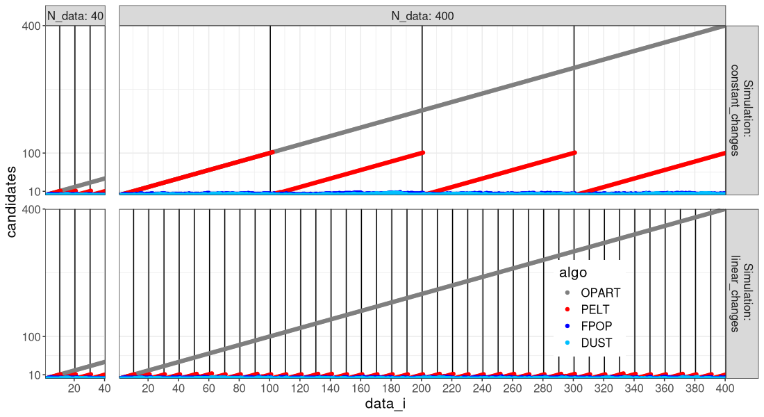
The figure above shows that DUST pruned much more than PELT, nearly the same amount as FPOP.
Heat maps
Another way to view this is by looking at the cost of each candidate change-point considered, as in the heat map below.
algo.levs <- c("OPART","PELT","FPOP","DUST")
(both_index <- addSim(rbindlist(both_index_list, use.names=TRUE))[, let(
  Algorithm = factor(algo, algo.levs)
)][])
##         N_data       simulation   algo data_i change_i       cost         Simulation Algorithm
##          <num>           <char> <char>  <int>    <num>      <num>             <char>    <fctr>
##      1:     40 constant_changes  OPART      1        1  -76.51163 \nconstant_changes     OPART
##      2:     40 constant_changes  OPART      2        1  -91.33987 \nconstant_changes     OPART
##      3:     40 constant_changes  OPART      2        2  -41.99613 \nconstant_changes     OPART
##      4:     40 constant_changes  OPART      3        1  -83.68055 \nconstant_changes     OPART
##      5:     40 constant_changes  OPART      3        2  -50.42746 \nconstant_changes     OPART
##     ---
## 191072:    400   linear_changes   DUST    396      391 -130.71096   \nlinear_changes      DUST
## 191073:    400   linear_changes   DUST    397      391 -130.71096   \nlinear_changes      DUST
## 191074:    400   linear_changes   DUST    398      391 -130.71096   \nlinear_changes      DUST
## 191075:    400   linear_changes   DUST    399      391 -130.71096   \nlinear_changes      DUST
## 191076:    400   linear_changes   DUST    400      391 -130.71096   \nlinear_changes      DUST
for(a in algo.levs){
  gg <- ggplot()+
    ggtitle(a)+
    theme_bw()+
    theme(
      text=element_text(size=20))+
    coord_equal()+
    geom_tile(aes(
      data_i, change_i, fill=cost),
      data=both_index[Algorithm==a])+
    scale_fill_gradient(low="black", high="red")+
    facet_grid(Simulation ~ N_data, label=label_both)
  print(gg)
}
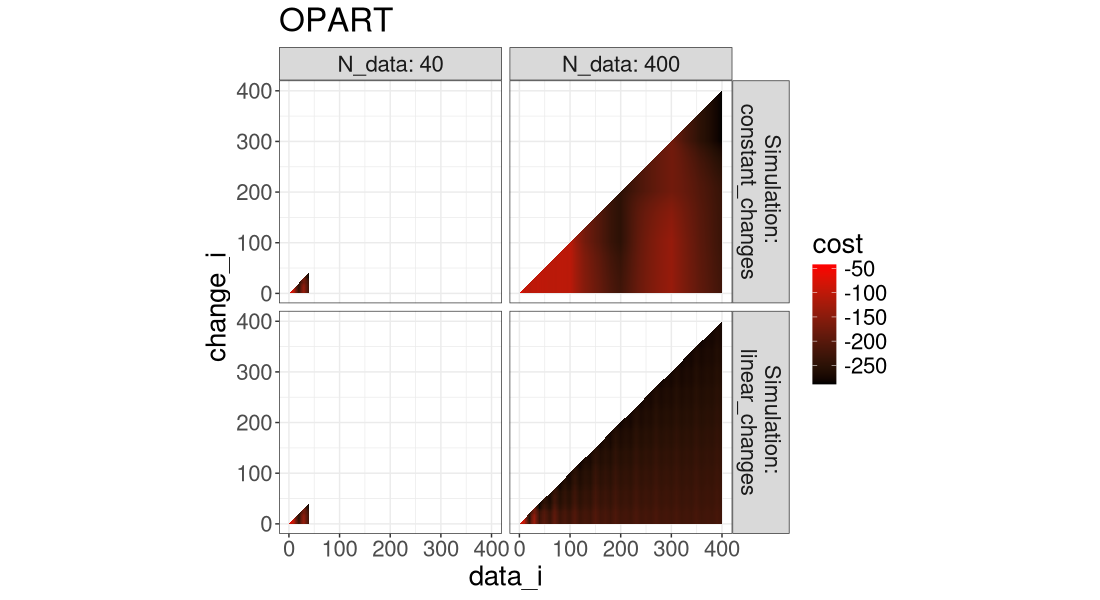
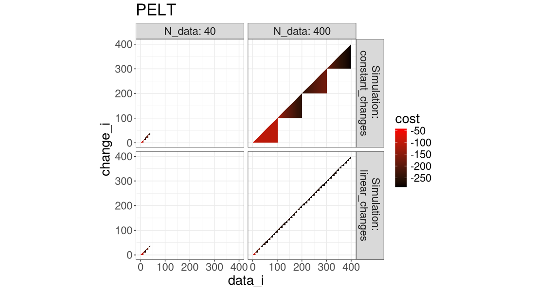
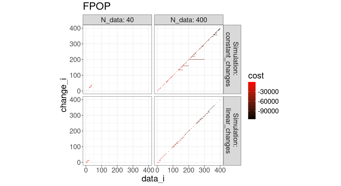
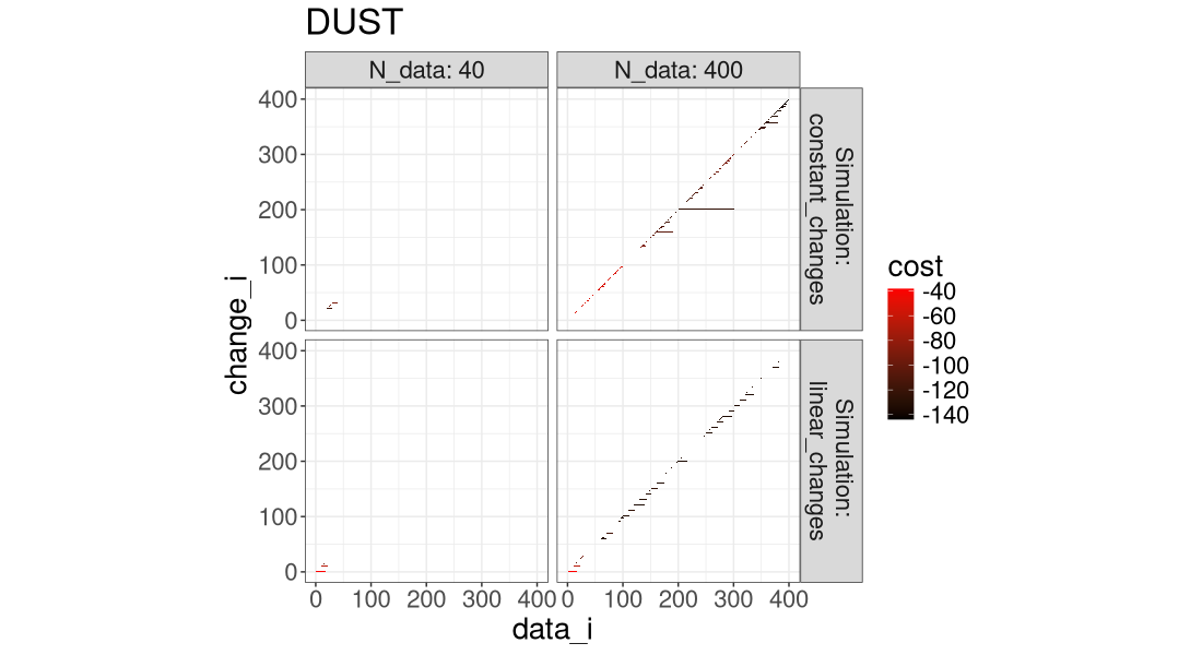
Another way to visualize it is in the plot below, which super-imposes the three algos.
ggplot()+
  theme_bw()+
  theme(
    legend.position=c(0.8, 0.2),
    text=element_text(size=15))+
  geom_tile(aes(
    data_i, change_i, fill=Algorithm),
    data=both_index)+
  scale_fill_manual(values=algo.colors)+
  scale_x_continuous(
    breaks=seq(0,max(N_data_vec),by=20))+
  facet_grid(Simulation ~ N_data, label=label_both, scales="free", space="free")
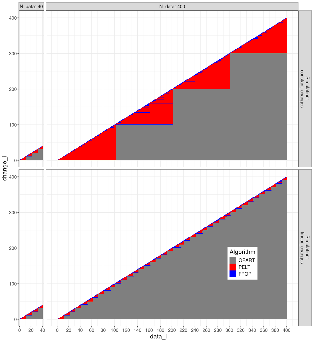
It is clear that FPOP/DUST prune much more than PELT, especially in the case of constant changes (segments that get larger with the overall number of data).
Double check FPOP for constant changes
Before running a simulation on varying data sizes, here we check that the penalty value results in the right number of change-points, for a larger data set.
N_data <- 1e5
sim_fun <- sim_fun_list$constant_changes
data_mean_vec <- sim_fun(N_data)
set.seed(1)
data_value <- rnorm(N_data, data_mean_vec, 2)
wfit <- fpopw::Fpop(data_value, penalty)
dfit <- dust::dust.1D(data_value, penalty)
rbind(
  FPOP=wfit$t.est,
  DUST=dfit$changepoints)
##       [,1]  [,2]  [,3]  [,4]
## FPOP 25000 50000 75000 1e+05
## DUST 25000 50000 75000 1e+05
The result above shows that there are four segments detected (three change-points), which is the expected number in our “constant changes” simulation.
atime comparison
The atime() function can be used to perform asymptotic time/memory/etc comparisons.
This means that we will increase N, and monitor how fast certain quantities grow with N.
We begin by defining the data sizes N of interest:
base_N <- c(100,200,400,800)
(all_N <- unlist(lapply(10^seq(0,5), function(x)x*base_N)))
##  [1] 1e+02 2e+02 4e+02 8e+02 1e+03 2e+03 4e+03 8e+03 1e+04 2e+04 4e+04 8e+04 1e+05 2e+05 4e+05 8e+05 1e+06 2e+06 4e+06
## [20] 8e+06 1e+07 2e+07 4e+07 8e+07
The data sizes above are on a log scale between 10 and 1,000,000. Next, we define a list that enumerates the different combinations in the experiment.
grid_args <- list(
  list(simulation=names(sim_fun_list)),
  DUST=quote({
    dfit <- dust::dust.1D(data_list[[simulation]], penalty)
    with(dfit, data.frame(
      mean_candidates=mean(nb),
      segments=length(changepoints),
      max_seg_size=max(diff(c(0,changepoints)))))
  }),
  FPOP=quote({
    pfit <- fpopw::Fpop(
      data_list[[simulation]], penalty, verbose_file=tempfile())
    count_dt <- pfit$model[, .(intervals=.N), by=data_i]
    data.frame(
      mean_candidates=mean(count_dt$intervals),
      segments=length(pfit$t.est),
      max_seg_size=max(diff(c(0,pfit$t.est))))
  }))
for(algo in names(algo.prune)){
  prune <- algo.prune[[algo]]
  grid_args[[algo]] <- substitute({
    data_value <- data_list[[simulation]]
    fit <- PELT(data_value, penalty, prune=prune)
    dec <- decode(fit$change)
    data.frame(
      mean_candidates=mean(fit$candidates),
      segments=nrow(dec),
      max_seg_size=max(diff(c(0,dec$last.i))))
  }, list(prune=prune))
}
(expr.list <- do.call(atime::atime_grid, grid_args))
## $`DUST simulation=constant_changes`
## {
##     dfit <- dust::dust.1D(data_list[["constant_changes"]], penalty)
##     with(dfit, data.frame(mean_candidates = mean(nb), segments = length(changepoints),
##         max_seg_size = max(diff(c(0, changepoints)))))
## }
##
## $`DUST simulation=linear_changes`
## {
##     dfit <- dust::dust.1D(data_list[["linear_changes"]], penalty)
##     with(dfit, data.frame(mean_candidates = mean(nb), segments = length(changepoints),
##         max_seg_size = max(diff(c(0, changepoints)))))
## }
##
## $`FPOP simulation=constant_changes`
## {
##     pfit <- fpopw::Fpop(data_list[["constant_changes"]], penalty,
##         verbose_file = tempfile())
##     count_dt <- pfit$model[, .(intervals = .N), by = data_i]
##     data.frame(mean_candidates = mean(count_dt$intervals), segments = length(pfit$t.est),
##         max_seg_size = max(diff(c(0, pfit$t.est))))
## }
##
## $`FPOP simulation=linear_changes`
## {
##     pfit <- fpopw::Fpop(data_list[["linear_changes"]], penalty,
##         verbose_file = tempfile())
##     count_dt <- pfit$model[, .(intervals = .N), by = data_i]
##     data.frame(mean_candidates = mean(count_dt$intervals), segments = length(pfit$t.est),
##         max_seg_size = max(diff(c(0, pfit$t.est))))
## }
##
## $`OPART simulation=constant_changes`
## {
##     data_value <- data_list[["constant_changes"]]
##     fit <- PELT(data_value, penalty, prune = FALSE)
##     dec <- decode(fit$change)
##     data.frame(mean_candidates = mean(fit$candidates), segments = nrow(dec),
##         max_seg_size = max(diff(c(0, dec$last.i))))
## }
##
## $`OPART simulation=linear_changes`
## {
##     data_value <- data_list[["linear_changes"]]
##     fit <- PELT(data_value, penalty, prune = FALSE)
##     dec <- decode(fit$change)
##     data.frame(mean_candidates = mean(fit$candidates), segments = nrow(dec),
##         max_seg_size = max(diff(c(0, dec$last.i))))
## }
##
## $`PELT simulation=constant_changes`
## {
##     data_value <- data_list[["constant_changes"]]
##     fit <- PELT(data_value, penalty, prune = TRUE)
##     dec <- decode(fit$change)
##     data.frame(mean_candidates = mean(fit$candidates), segments = nrow(dec),
##         max_seg_size = max(diff(c(0, dec$last.i))))
## }
##
## $`PELT simulation=linear_changes`
## {
##     data_value <- data_list[["linear_changes"]]
##     fit <- PELT(data_value, penalty, prune = TRUE)
##     dec <- decode(fit$change)
##     data.frame(mean_candidates = mean(fit$candidates), segments = nrow(dec),
##         max_seg_size = max(diff(c(0, dec$last.i))))
## }
##
## attr(,"parameters")
##                            expr.name expr.grid       simulation
##                               <char>    <char>           <char>
## 1:  DUST simulation=constant_changes      DUST constant_changes
## 2:    DUST simulation=linear_changes      DUST   linear_changes
## 3:  FPOP simulation=constant_changes      FPOP constant_changes
## 4:    FPOP simulation=linear_changes      FPOP   linear_changes
## 5: OPART simulation=constant_changes     OPART constant_changes
## 6:   OPART simulation=linear_changes     OPART   linear_changes
## 7:  PELT simulation=constant_changes      PELT constant_changes
## 8:    PELT simulation=linear_changes      PELT   linear_changes
Above we see a list with 8 expressions to run, and a data table with the corresponding number of rows. Note that each expression
- returns a data frame with one row and three columns that will be used as units to analyze as a function of N.
- should depend on data size N, which does not appear in the
expressions above, but it is used to define
data_listin thesetupargument below:
cache.rds <- "2025-04-15-PELT-vs-fpopw.rds"
if(file.exists(cache.rds)){
  atime_list <- readRDS(cache.rds)
}else{
  atime_list <- atime::atime(
    N=all_N,
    setup={
      data_list <- list()
      for(simulation in names(sim_fun_list)){
        sim_fun <- sim_fun_list[[simulation]]
        data_mean_vec <- sim_fun(N)
        set.seed(1)
        data_list[[simulation]] <- rnorm(N, data_mean_vec, 2)
      }
    },
    expr.list=expr.list,
    seconds.limit=1,
    result=TRUE)
  saveRDS(atime_list, cache.rds)
}
Note in the code above that we run the timing inside if(file.exists, which is a caching mechanism.
The result is time-consuming to compute, so the first time it is computed, it is saved to disk as an RDS file, and then subsequently read from disk, to save time.
Finally, we plot the different units as a function of data size N, in the figure below.
refs_list <- atime::references_best(atime_list)
ggplot()+
  theme(text=element_text(size=12))+
  directlabels::geom_dl(aes(
    N, empirical, color=expr.grid, label=expr.grid),
    data=refs_list$measurements,
    method="right.polygons")+
  geom_line(aes(
    N, empirical, color=expr.grid),
    data=refs_list$measurements)+
  scale_color_manual(
    "algorithm",
    guide="none",
    values=algo.colors)+
  facet_grid(unit ~ simulation, scales="free")+
  scale_x_log10(
    "N = number of data in sequence",
    breaks=10^seq(2,6),
    limits=c(NA, 1e8))+
  scale_y_log10("")
Above the figure shows a different curve for each algorithm, and a different panel for each simulation and measurement unit. We can observe that
- PELT memory usage in kilobytes has a larger slope for constant changes, than for linear changes. This implies a larger asymptotic complexity class.
- The maximum segment size,
max_seg_size, is the same for all algos, indicating that the penalty was chosen appropriately, and the algorithms are computing the same optimal solution. - Similarly, the mean number of candidates considered by the PELT algorithm has a larger slope for constant changes (same as OPART/linear in N), than for linear changes (relatively constant).
- For PELT seconds, we see a slightly larger slope for seconds in constant changes, compared to linear changes.
- As expected, number of
segmentsis constant for a constant number of changes (left), and increasing for a linear number of changes (right).
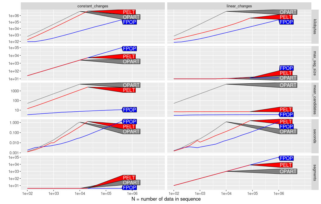
Below we plot the same data in a different way, that facilitates comparisons across the type of simulation:
refs_list$meas[, let(
  Simulation = sub("_","\n",simulation),
  Algorithm = factor(expr.grid, algo.levs)
)][]
##              unit                         expr.name fun.name fun.latex expr.grid       simulation     N          min
##            <char>                            <char>   <char>    <char>    <char>           <char> <num>        <num>
##   1:    kilobytes  DUST simulation=constant_changes        N         N      DUST constant_changes 1e+02 0.0003440930
##   2:    kilobytes    DUST simulation=linear_changes        N         N      DUST   linear_changes 1e+02 0.0003319740
##   3:    kilobytes  FPOP simulation=constant_changes  N log N N \\log N      FPOP constant_changes 1e+02 0.0010634530
##   4:    kilobytes    FPOP simulation=linear_changes        N         N      FPOP   linear_changes 1e+02 0.0008895912
##   5:    kilobytes OPART simulation=constant_changes      N^2       N^2     OPART constant_changes 1e+02 0.0012234050
##  ---
## 551: max_seg_size    DUST simulation=linear_changes     <NA>      <NA>      DUST   linear_changes 2e+06 0.1745800580
## 552: max_seg_size  DUST simulation=constant_changes        N         N      DUST constant_changes 4e+06 1.4330559800
## 553: max_seg_size    DUST simulation=linear_changes     <NA>      <NA>      DUST   linear_changes 4e+06 0.3500808589
## 554: max_seg_size    DUST simulation=linear_changes     <NA>      <NA>      DUST   linear_changes 8e+06 0.7785552479
## 555: max_seg_size    DUST simulation=linear_changes     <NA>      <NA>      DUST   linear_changes 1e+07 0.9580125660
##            median      itr/sec    gc/sec n_itr  n_gc            result
##             <num>        <num>     <num> <int> <num>            <list>
##   1: 0.0003712554 2454.4469723 0.0000000    10     0 <data.frame[1x3]>
##   2: 0.0003471415 2756.5684704 0.0000000    10     0 <data.frame[1x3]>
##   3: 0.0013680826  671.6772182 0.0000000    10     0 <data.frame[1x3]>
##   4: 0.0009680756 1045.1979132 0.0000000    10     0 <data.frame[1x3]>
##   5: 0.0013303495  748.7730286 0.0000000    10     0 <data.frame[1x3]>
##  ---
## 551: 0.1790242815    5.6581400 5.6581400     5     5 <data.frame[1x3]>
## 552: 1.4663964449    0.6724955 0.7397451    10    11 <data.frame[1x3]>
## 553: 0.3759252669    2.4664677 2.9597613    10    12 <data.frame[1x3]>
## 554: 0.9063347740    1.1508771 1.8414033    10    16 <data.frame[1x3]>
## 555: 1.1294077394    0.9009359 1.8919653    10    21 <data.frame[1x3]>
##                                                                                   time             gc    kilobytes
##                                                                                 <list>         <list>        <num>
##   1: 0.0006167080,0.0004174080,0.0003564690,0.0003697509,0.0004268159,0.0004773060,... <tbl_df[10x3]> 3.585938e+00
##   2: 0.0005097550,0.0003699249,0.0003539650,0.0003345360,0.0003319740,0.0003563149,... <tbl_df[10x3]> 3.585938e+00
##   3:       0.001563062,0.001173103,0.001144646,0.001063453,0.001070530,0.002711618,... <tbl_df[10x3]> 7.002344e+01
##   4: 0.0009703070,0.0009962391,0.0009237260,0.0008895912,0.0008919862,0.0010226031,... <tbl_df[10x3]> 6.784375e+01
##   5:       0.001551917,0.001356952,0.001350875,0.001369654,0.001245563,0.001309824,... <tbl_df[10x3]> 5.912969e+02
##  ---
## 551:                   0.1783938,0.1756855,0.1833944,0.1785470,0.1753685,0.1812852,... <tbl_df[10x3]> 7.500102e+04
## 552:                         1.475066,1.493653,1.457727,1.562417,1.433056,1.450362,... <tbl_df[10x3]> 1.250020e+05
## 553:                   0.3943201,0.4729741,0.3504990,0.4880445,0.3529972,0.4573742,... <tbl_df[10x3]> 1.500010e+05
## 554:                   0.8952151,0.7785552,0.9344374,0.7881498,0.9174544,0.9198045,... <tbl_df[10x3]> 3.000008e+05
## 555:                         1.235551,1.008993,1.220231,1.120291,1.015123,1.138524,... <tbl_df[10x3]> 3.750010e+05
##               q25          q75         max         mean           sd mean_candidates segments max_seg_size
##             <num>        <num>       <num>        <num>        <num>           <num>    <int>        <num>
##   1: 0.0003498269 0.0004244639 0.000616708 0.0004074238 8.551939e-05        1.970000        4           25
##   2: 0.0003374740 0.0003557274 0.000509755 0.0003627699 5.299184e-05        1.760000       10           10
##   3: 0.0011483961 0.0016439211 0.002711618 0.0014888104 5.040464e-04        3.370000        4           25
##   4: 0.0009274510 0.0009892038 0.001022603 0.0009567566 4.471803e-05        2.910000       10           10
##   5: 0.0012891432 0.0013590138 0.001551917 0.0013355182 9.083811e-05       50.500000        4           25
##  ---
## 551: 0.1763625847 0.1809086355 0.190087997 0.1796623020 4.573240e-03        1.832713   200000           14
## 552: 1.4518229705 1.5303621150 1.562417001 1.4869987807 4.971707e-02       16.791806        4      1000000
## 553: 0.3533985880 0.4690741207 0.488044514 0.4054381033 6.045301e-02        1.832841   399999           20
## 554: 0.7955587294 0.9239733572 0.934437368 0.8689025400 6.743490e-02        1.833660   799997           20
## 555: 1.0176718701 1.1890061875 1.235550567 1.1099569251 1.003971e-01        1.833507   999996           20
##                                     expr.class                                       expr.latex    empirical
##                                         <char>                                           <char>        <num>
##   1:       DUST simulation=constant_changes\nN         DUST simulation=constant_changes\n$O(N)$ 3.585938e+00
##   2:         DUST simulation=linear_changes\nN           DUST simulation=linear_changes\n$O(N)$ 3.585938e+00
##   3: FPOP simulation=constant_changes\nN log N FPOP simulation=constant_changes\n$O(N \\log N)$ 7.002344e+01
##   4:         FPOP simulation=linear_changes\nN           FPOP simulation=linear_changes\n$O(N)$ 6.784375e+01
##   5:    OPART simulation=constant_changes\nN^2      OPART simulation=constant_changes\n$O(N^2)$ 5.912969e+02
##  ---
## 551:        DUST simulation=linear_changes\nNA          DUST simulation=linear_changes\n$O(NA)$ 1.400000e+01
## 552:       DUST simulation=constant_changes\nN         DUST simulation=constant_changes\n$O(N)$ 1.000000e+06
## 553:        DUST simulation=linear_changes\nNA          DUST simulation=linear_changes\n$O(NA)$ 2.000000e+01
## 554:        DUST simulation=linear_changes\nNA          DUST simulation=linear_changes\n$O(NA)$ 2.000000e+01
## 555:        DUST simulation=linear_changes\nNA          DUST simulation=linear_changes\n$O(NA)$ 2.000000e+01
##             Simulation Algorithm
##                 <char>    <fctr>
##   1: constant\nchanges      DUST
##   2:   linear\nchanges      DUST
##   3: constant\nchanges      FPOP
##   4:   linear\nchanges      FPOP
##   5: constant\nchanges     OPART
##  ---
## 551:   linear\nchanges      DUST
## 552: constant\nchanges      DUST
## 553:   linear\nchanges      DUST
## 554:   linear\nchanges      DUST
## 555:   linear\nchanges      DUST
ggplot()+
  theme(
    legend.position="none",
    text=element_text(size=12))+
  directlabels::geom_dl(aes(
    N, empirical, color=Simulation, label=Simulation),
    data=refs_list$measurements,
    method="right.polygons")+
  geom_line(aes(
    N, empirical, color=Simulation),
    data=refs_list$measurements)+
  facet_grid(unit ~ Algorithm, scales="free")+
  scale_x_log10(
    "N = number of data in sequence",
    breaks=10^seq(2,6),
    limits=c(NA, 1e8))+
  scale_y_log10("")
The plot above makes it easier to notice some interesting trends in the mean number of candidates:
- For PELT and FPOP the mean number of candidates is increases for a constant number of changes, but at different rates (FPOP much slower than PELT).
expr.levs <- CJ(
  algo=algo.levs,
  simulation=names(sim_fun_list)
)[algo.levs, paste0(algo,"\n",simulation), on="algo"]
edit_expr <- function(DT)DT[
, expr.name := factor(sub(" simulation=", "\n", expr.name), expr.levs)]
edit_expr(refs_list$meas)
edit_expr(refs_list$plot.ref)
plot(refs_list)+
  theme(panel.spacing=grid::unit(1.5,"lines"))
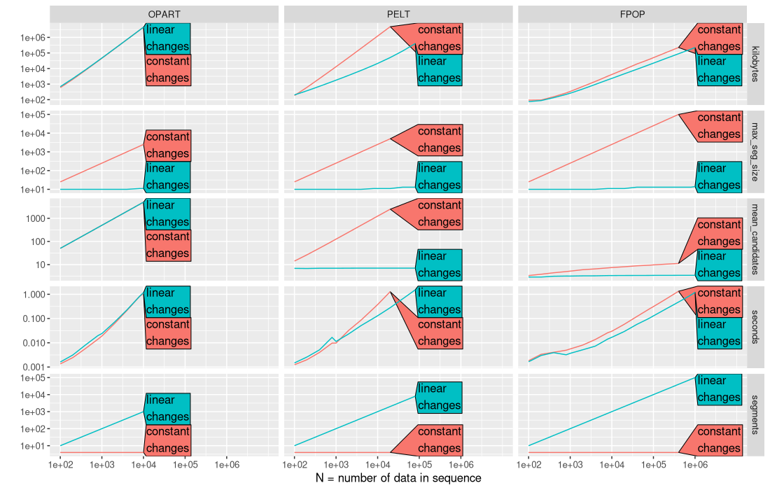
The plot above is an empirical verification of our earlier complexity claims.
- OPART
mean_candidatesis linear,O(N), and time and memory are quadratic,O(N^2). - PELT with constant changes has linear
mean_candidates,O(N), and quadratic time and memory,O(N^2)(same as OPART, no asymptotic speedup). - PELT with linear changes has sub-linear
mean_candidates(constant or log), and linear or log-linear time/memory. - FPOP always has sub-linear
mean_candidates(constant or log), and linear or log-linear time/memory.
The code/plot below shows the speedups in this case.
pred_list <- predict(refs_list)
ggplot()+
  theme_bw()+
  theme(text=element_text(size=20))+
  geom_line(aes(
    N, empirical, color=expr.grid),
    data=pred_list$measurements[unit=="seconds"])+
  directlabels::geom_dl(aes(
    N, unit.value, color=expr.grid, label=sprintf(
      "%s\n%s\nN=%s",
      expr.grid,
      ifelse(expr.grid %in% c("FPOP","DUST"), "C++", "R"),
      format(round(N), big.mark=",", scientific=FALSE, trim=TRUE))),
    data=pred_list$prediction,
    method=list(cex=1.5,directlabels::polygon.method("top",offset.cm = 0.5)))+
  scale_color_manual(
    "algorithm",
    guide="none",
    values=algo.colors)+
  facet_grid(. ~ simulation, scales="free", labeller=label_both)+
  scale_x_log10(
    "N = number of data in sequence",
    breaks=10^seq(2,7),
    limits=c(NA, 5e7))+
  scale_y_log10(
    "Computation time (seconds)",
    breaks=10^seq(-3,0),
    limits=10^c(-3,1))
## Warning: Removed 5 rows containing missing values or values outside the scale range (`geom_line()`).
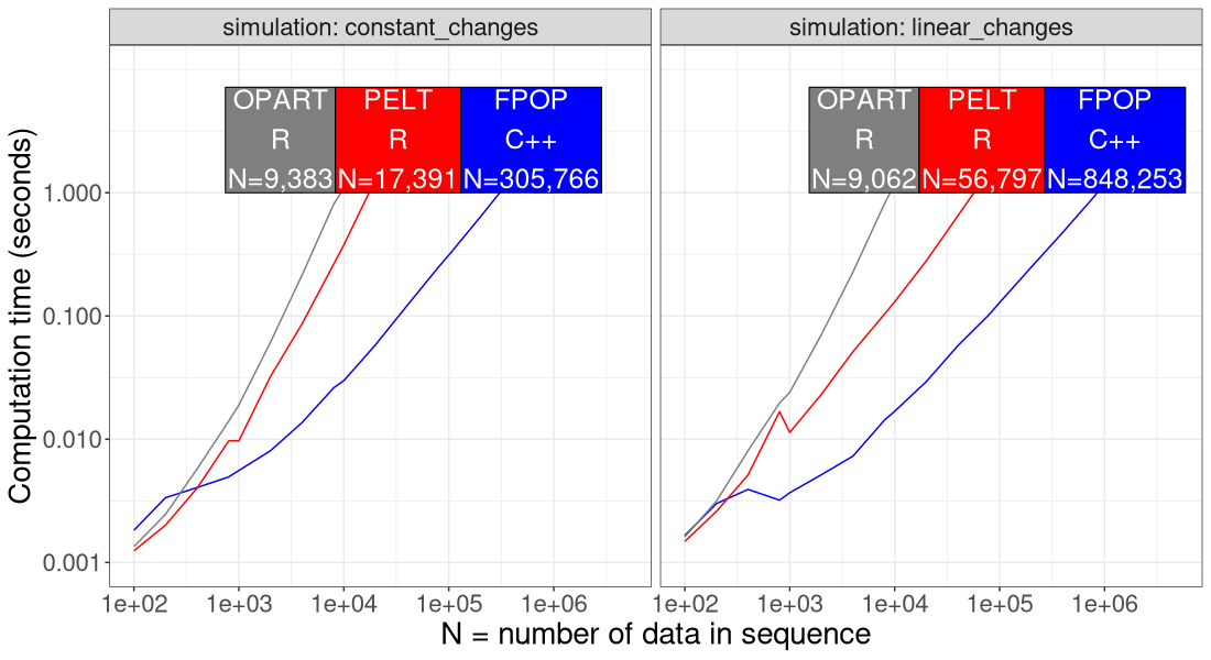
The figure above shows the throughput (data size N) which is possible to compute in 1 second using each algorithm. We see that FPOP is 10-100x faster than OPART/PELT. Part of the difference is that OPART/PELT were coded in R, whereas FPOP was coded in C++ (faster). Another difference is that FPOP is asymptotically faster with constant changes, as can be seen by a smaller slope for FPOP, compared to OPART/PELT.
Below we zoom in on the number of candidate change-points considered by each algorithm.
cand_dt <- pred_list$measurements[unit=="mean_candidates"]
ggplot()+
  theme_bw()+
  theme(text=element_text(size=20))+
  geom_line(aes(
    N, empirical, color=expr.grid),
    data=cand_dt)+
  directlabels::geom_dl(aes(
    N, empirical, color=expr.grid, label=expr.grid),
    data=cand_dt,
    method=list(cex=2, "right.polygons"))+
  scale_color_manual(
    "algorithm",
    guide="none",
    values=algo.colors)+
  facet_grid(. ~ simulation, scales="free", labeller=label_both)+
  scale_x_log10(
    "N = number of data in sequence",
    breaks=10^seq(2,7),
    limits=c(NA, 1e8))+
  scale_y_log10(
    "Mean number of candidate change-points",
    limits=10^c(0, 4))
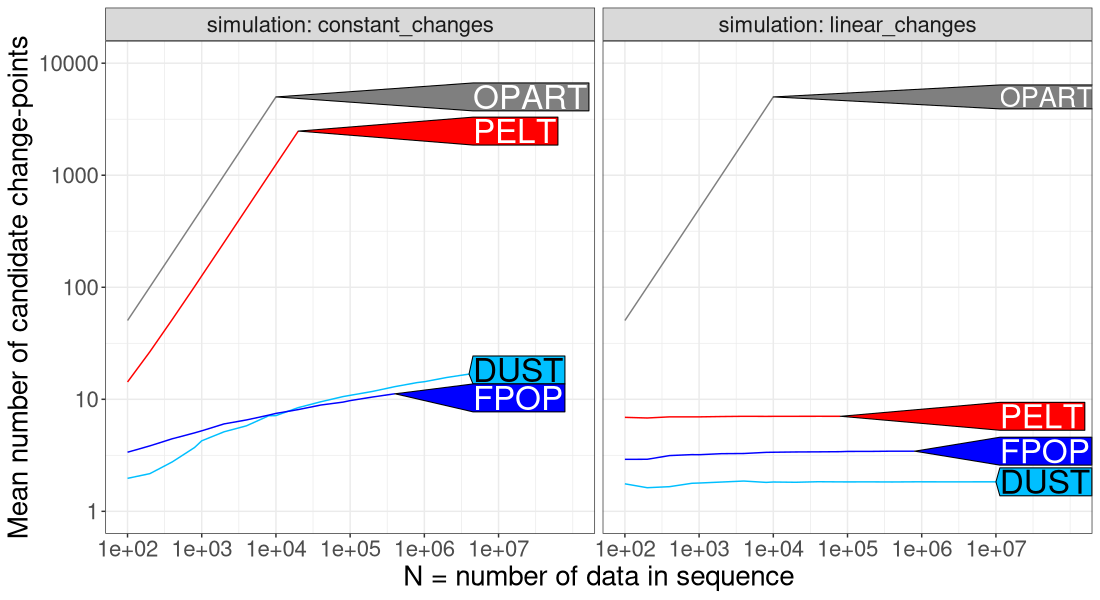
The figure above shows that
- OPART always considers a linear number of candidates (slow).
- PELT also considers a linear number of candidates (slow), when the number of changes is constant.
- PELT considers a sub-linear number of candidates (fast), when the number of changes is linear.
- FPOP always considers sub-linear number of candidates (fast), which is either constant for a linear number of changes, or logarithmic for a constant number of changes.
Conclusions
We have explored three algorithms for optimal change-point detection.
- The classic OPART algorithm is always quadratic time in the number of data to segment.
- The Pruned Exact Linear Time (PELT) algorithm can indeed be linear time in the number of data to segment, but only when the number of change-points grows with the number of data points. When the number of change-points is constant, there are ever-increasing segments, and the PELT algorithm must compute a cost for each candidate on these large segments; in this situation, PELT suffers from the same quadratic time complexity as OPART.
- The FPOP algorithm is fast (linear or log-linear) in both of the scenarios we examined.
Session info
sessionInfo()
## R Under development (unstable) (2025-05-21 r88220)
## Platform: x86_64-pc-linux-gnu
## Running under: Ubuntu 24.04.2 LTS
##
## Matrix products: default
## BLAS:   /usr/lib/x86_64-linux-gnu/blas/libblas.so.3.12.0
## LAPACK: /usr/lib/x86_64-linux-gnu/lapack/liblapack.so.3.12.0  LAPACK version 3.12.0
##
## locale:
##  [1] LC_CTYPE=fr_FR.UTF-8       LC_NUMERIC=C               LC_TIME=fr_FR.UTF-8        LC_COLLATE=fr_FR.UTF-8
##  [5] LC_MONETARY=fr_FR.UTF-8    LC_MESSAGES=fr_FR.UTF-8    LC_PAPER=fr_FR.UTF-8       LC_NAME=C
##  [9] LC_ADDRESS=C               LC_TELEPHONE=C             LC_MEASUREMENT=fr_FR.UTF-8 LC_IDENTIFICATION=C
##
## time zone: Europe/Paris
## tzcode source: system (glibc)
##
## attached base packages:
## [1] stats     graphics  grDevices utils     datasets  methods   base
##
## other attached packages:
## [1] mlr3resampling_2025.6.23 mlr3_1.0.0.9000          future_1.58.0            ggplot2_3.5.1
## [5] data.table_1.17.99
##
## loaded via a namespace (and not attached):
##  [1] tidyselect_1.2.1       dust_0.3.0             dplyr_1.1.4            farver_2.1.2           filelock_1.0.3
##  [6] fastmap_1.2.0          promises_1.3.2         paradox_1.0.1          digest_0.6.37          rpart_4.1.24
## [11] base64url_1.4          mime_0.13              lifecycle_1.0.4        ellipsis_0.3.2         processx_3.8.6
## [16] magrittr_2.0.3         compiler_4.6.0         rlang_1.1.6            progress_1.2.3         tools_4.6.0
## [21] knitr_1.50             prettyunits_1.2.0      labeling_0.4.3         brew_1.0-10            htmlwidgets_1.6.4
## [26] pkgbuild_1.4.7         curl_6.2.2             plyr_1.8.9             batchtools_0.9.17      pkgload_1.4.0
## [31] miniUI_0.1.1.1         withr_3.0.2            purrr_1.0.4            mlr3misc_0.18.0        desc_1.4.3
## [36] grid_4.6.0             urlchecker_1.0.1       profvis_0.4.0          mlr3measures_1.0.0     xtable_1.8-4
## [41] colorspace_2.1-1       globals_0.18.0         scales_1.3.0           cli_3.6.5              crayon_1.5.3
## [46] generics_0.1.3         remotes_2.5.0          future.apply_1.20.0    directlabels_2025.5.20 sessioninfo_1.2.3
## [51] atime_2025.5.24        cachem_1.1.0           parallel_4.6.0         fpopw_1.2              vctrs_0.6.5
## [56] devtools_2.4.5         animint2_2025.6.4      callr_3.7.6            hms_1.1.3              listenv_0.9.1
## [61] lgr_0.4.4              glue_1.8.0             parallelly_1.45.0      RJSONIO_1.3-1.9        codetools_0.2-20
## [66] ps_1.9.1               stringi_1.8.7          gtable_0.3.6           later_1.4.1            quadprog_1.5-8
## [71] palmerpenguins_0.1.1   munsell_0.5.1          tibble_3.2.1           pillar_1.10.2          rappdirs_0.3.3
## [76] htmltools_0.5.8.1      R6_2.6.1               lattice_0.22-7         evaluate_1.0.3         shiny_1.10.0
## [81] backports_1.5.0        memoise_2.0.1          httpuv_1.6.15          Rcpp_1.0.14            uuid_1.2-1
## [86] checkmate_2.3.2        xfun_0.51              fs_1.6.6               usethis_3.1.0          pkgconfig_2.0.3