Comparing pruning methods for optimal partitioning
The goal of this post is to compare two pruning methods for speeding up the optimal partitioning algorithm.
- We assume that we want to find change-points in a sequence of
Ndata. - All algorithms discussed are instances of dynamic programming, which
has a for loop over all
Ndata. In each iteration, the algorithm considers a certain number of candidate change-pointsC(on average). The algorithm is overallO(NC)time. - Optimal partitioning (OPART) computes the best segmentation for a
given loss function, data sequence, and non-negative penalty
value. Each iteration considers the loss for each previous candidate
change-point,
C=O(N)linear time per iteration, which implies quadraticO(N^2)time overall. - Pruned Exact Linear Time (PELT) reduces the number of candidate
change-points that must be considered at each iteration, from the
whole data sequence size
N, to the size of a segmentS, soC=O(S). This gives an algorithm which isO(NS)time overall.- If the number of change-points grows linearly with the data size
N, then the segment size is constant,S=O(1)with respect to number of dataN, and the PELT algorithm is indeed linear time overall,O(N). - However in the case of a constant number of change-points, with
segment sizes that grow with the data sequence,
S=O(N)implies quadratic time overall,O(N^2).
- If the number of change-points grows linearly with the data size
- Functional Pruning Optimal Partitioning (FPOP) reduces the number of
candidate change-points to a number which is always less than the
number considered by PELT (see Maidstone 2017 paper for detailed
proof). The goal of this post is to show that it prunes more than
PELT in both cases:
- If the number of change-points grows linearly with the data size
N, then both PELT and FPOP areO(N)overall. - If the number of change-points is constant with respect to data
size
N, then FPOP considers onlyS=O(log N)change-points (empirically), which gives an algorithm that isO(N log N), log-linear time overall.
- If the number of change-points grows linearly with the data size
Simulate data sequences
We simulate data in two scenarios: linear and constant number of changes.
mean_vec <- c(10,20,5,25)
sim_fun_list <- list(
  constant_changes=function(N){
    rep(mean_vec, each=N/4)
  },
  linear_changes=function(N){
    rep(rep(mean_vec, each=25), l=N)
  })
lapply(sim_fun_list, function(f)f(100))
## $constant_changes
##   [1] 10 10 10 10 10 10 10 10 10 10 10 10 10 10 10 10 10 10 10 10 10 10 10 10 10 20 20 20 20 20 20 20 20 20 20 20 20 20
##  [39] 20 20 20 20 20 20 20 20 20 20 20 20  5  5  5  5  5  5  5  5  5  5  5  5  5  5  5  5  5  5  5  5  5  5  5  5  5 25
##  [77] 25 25 25 25 25 25 25 25 25 25 25 25 25 25 25 25 25 25 25 25 25 25 25 25
##
## $linear_changes
##   [1] 10 10 10 10 10 10 10 10 10 10 10 10 10 10 10 10 10 10 10 10 10 10 10 10 10 20 20 20 20 20 20 20 20 20 20 20 20 20
##  [39] 20 20 20 20 20 20 20 20 20 20 20 20  5  5  5  5  5  5  5  5  5  5  5  5  5  5  5  5  5  5  5  5  5  5  5  5  5 25
##  [77] 25 25 25 25 25 25 25 25 25 25 25 25 25 25 25 25 25 25 25 25 25 25 25 25
As can be seen above, both functions return a vector of values that represent the true segment mean. Below we use both functions with a three different data sizes.
library(data.table)
N_data_vec <- c(100,200,400)
sim_data_list <- list()
sim_changes_list <- list()
for(N_data in N_data_vec){
  for(simulation in names(sim_fun_list)){
    sim_fun <- sim_fun_list[[simulation]]
    data_mean_vec <- sim_fun(N_data)
    end <- which(diff(data_mean_vec) != 0)
    set.seed(1)
    data_value <- rpois(N_data, data_mean_vec)
    sim_data_list[[paste(N_data, simulation)]] <- data.table(
      N_data, simulation, data_index=seq_along(data_value), data_value)
    sim_changes_list[[paste(N_data, simulation)]] <- data.table(
      N_data, simulation, end)
  }
}
addSim <- function(DT)DT[, Simulation := paste0("\n", simulation)][]
(sim_changes <- addSim(rbindlist(sim_changes_list)))
##     N_data       simulation   end         Simulation
##      <num>           <char> <int>             <char>
##  1:    100 constant_changes    25 \nconstant_changes
##  2:    100 constant_changes    50 \nconstant_changes
##  3:    100 constant_changes    75 \nconstant_changes
##  4:    100   linear_changes    25   \nlinear_changes
##  5:    100   linear_changes    50   \nlinear_changes
##  6:    100   linear_changes    75   \nlinear_changes
##  7:    200 constant_changes    50 \nconstant_changes
##  8:    200 constant_changes   100 \nconstant_changes
##  9:    200 constant_changes   150 \nconstant_changes
## 10:    200   linear_changes    25   \nlinear_changes
## 11:    200   linear_changes    50   \nlinear_changes
## 12:    200   linear_changes    75   \nlinear_changes
## 13:    200   linear_changes   100   \nlinear_changes
## 14:    200   linear_changes   125   \nlinear_changes
## 15:    200   linear_changes   150   \nlinear_changes
## 16:    200   linear_changes   175   \nlinear_changes
## 17:    400 constant_changes   100 \nconstant_changes
## 18:    400 constant_changes   200 \nconstant_changes
## 19:    400 constant_changes   300 \nconstant_changes
## 20:    400   linear_changes    25   \nlinear_changes
## 21:    400   linear_changes    50   \nlinear_changes
## 22:    400   linear_changes    75   \nlinear_changes
## 23:    400   linear_changes   100   \nlinear_changes
## 24:    400   linear_changes   125   \nlinear_changes
## 25:    400   linear_changes   150   \nlinear_changes
## 26:    400   linear_changes   175   \nlinear_changes
## 27:    400   linear_changes   200   \nlinear_changes
## 28:    400   linear_changes   225   \nlinear_changes
## 29:    400   linear_changes   250   \nlinear_changes
## 30:    400   linear_changes   275   \nlinear_changes
## 31:    400   linear_changes   300   \nlinear_changes
## 32:    400   linear_changes   325   \nlinear_changes
## 33:    400   linear_changes   350   \nlinear_changes
## 34:    400   linear_changes   375   \nlinear_changes
##     N_data       simulation   end         Simulation
Above we see the table of simulated change-points.
- For
constant_changessimulation, there are always 3 change-points. - For
linear_changessimulation, there are more change-points when there are more data.
Below we visualize the simulated data.
(sim_data <- addSim(rbindlist(sim_data_list)))
##       N_data       simulation data_index data_value         Simulation
##        <num>           <char>      <int>      <int>             <char>
##    1:    100 constant_changes          1          8 \nconstant_changes
##    2:    100 constant_changes          2         10 \nconstant_changes
##    3:    100 constant_changes          3          7 \nconstant_changes
##    4:    100 constant_changes          4         11 \nconstant_changes
##    5:    100 constant_changes          5         14 \nconstant_changes
##   ---
## 1396:    400   linear_changes        396         24   \nlinear_changes
## 1397:    400   linear_changes        397         20   \nlinear_changes
## 1398:    400   linear_changes        398         22   \nlinear_changes
## 1399:    400   linear_changes        399         21   \nlinear_changes
## 1400:    400   linear_changes        400         23   \nlinear_changes
library(ggplot2)
ggplot()+
  theme_bw()+
  theme(text=element_text(size=14))+
  geom_vline(aes(
    xintercept=end+0.5),
    data=sim_changes)+
  geom_point(aes(
    data_index, data_value),
    color="grey50",
    data=sim_data)+
  facet_grid(Simulation ~ N_data, labeller=label_both, scales="free_x", space="free")+
  scale_x_continuous(
    breaks=seq(0,max(N_data_vec),by=50))
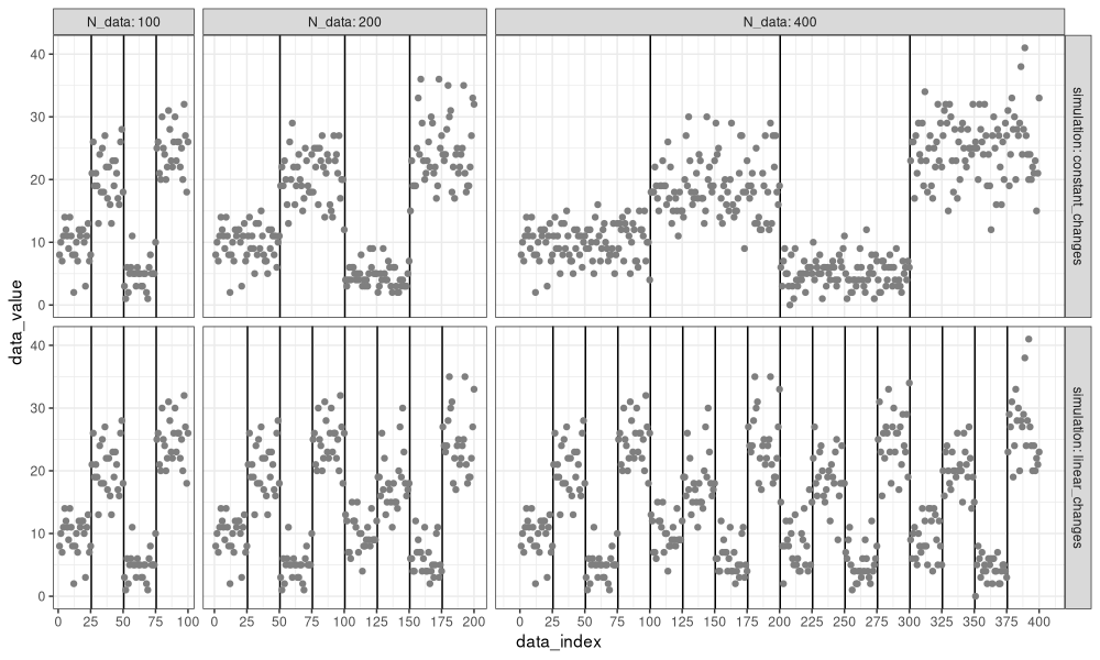
We see in the figure above that the data are the same in the two simulations, when there are only 100 data points. However, when there are 200 or 400 data, we see a difference:
- For the
constant_changessimulation, the number of change-points is still three (change-point every quarter of the data). - For the
linear_changessimulation, the number of change-points has increased from 3 to 7 to 15 (change-point every 25 data points).
PELT
Below we define a function which implements PELT for the Poisson loss, because we used a count data simulation above.
PELT <- function(sim.mat, penalty, prune=TRUE, verbose=FALSE){
  if(!is.matrix(sim.mat))sim.mat <- cbind(sim.mat)
  cum.data <- rbind(0, apply(sim.mat, 2, cumsum))
  sum_trick <- function(m, start, end)m[end+1,,drop=FALSE]-m[start,,drop=FALSE]
  cost_trick <- function(start, end){
    sum_vec <- sum_trick(cum.data, start, end)
    N <- end+1-start
    mean_vec <- sum_vec/N
    ifelse(sum_vec==0, 0, sum_vec*(1-log(mean_vec)))
  }
  N.data <- nrow(sim.mat)
  pelt.change.vec <- rep(NA_integer_, N.data)
  pelt.cost.vec <- rep(NA_real_, N.data+1)
  pelt.cost.vec[1] <- -penalty
  pelt.candidates.vec <- rep(NA_integer_, N.data)
  candidate.vec <- 1L
  if(verbose)index_dt_list <- list()
  for(up.to in 1:N.data){
    N.cand <- length(candidate.vec)
    pelt.candidates.vec[up.to] <- N.cand
    last.seg.cost <- rowSums(cost_trick(candidate.vec, rep(up.to, N.cand)))
    prev.cost <- pelt.cost.vec[candidate.vec]
    cost.no.penalty <- prev.cost+last.seg.cost
    total.cost <- cost.no.penalty+penalty
    if(verbose)index_dt_list[[up.to]] <- data.table(
      data_index=up.to, change=candidate.vec, cost=total.cost/up.to)
    best.i <- which.min(total.cost)
    pelt.change.vec[up.to] <- candidate.vec[best.i]
    total.cost.best <- total.cost[best.i]
    pelt.cost.vec[up.to+1] <- total.cost.best
    keep <- if(isTRUE(prune))cost.no.penalty < total.cost.best else TRUE
    candidate.vec <- c(candidate.vec[keep], up.to+1L)
  }
  list(
    change=pelt.change.vec,
    cost=pelt.cost.vec,
    candidates=pelt.candidates.vec,
    index_dt=if(verbose)rbindlist(index_dt_list))
}
decode <- function(best.change){
  seg.dt.list <- list()
  last.i <- length(best.change)
  while(last.i>0){
    first.i <- best.change[last.i]
    seg.dt.list[[paste(last.i)]] <- data.table(
      first.i, last.i)
    last.i <- first.i-1L
  }
  rbindlist(seg.dt.list)[seq(.N,1)]
}
pelt_info_list <- list()
pelt_segs_list <- list()
both_index_list <- list()
penalty <- 10
algo.prune <- c(
  OPART=FALSE,
  PELT=TRUE)
for(N_data in N_data_vec){
  for(simulation in names(sim_fun_list)){
    N_sim <- paste(N_data, simulation)
    data_value <- sim_data_list[[N_sim]]$data_value
    for(algo in names(algo.prune)){
      prune <- algo.prune[[algo]]
      fit <- PELT(data_value, penalty=penalty, prune=prune, verbose = TRUE)
      both_index_list[[paste(N_data, simulation, algo)]] <- data.table(
        N_data, simulation, algo, fit$index_dt)
      fit_seg_dt <- decode(fit$change)
      pelt_info_list[[paste(N_data,simulation,algo)]] <- data.table(
        N_data,simulation,algo,
        candidates=fit$candidates,data_index=seq_along(data_value))
      pelt_segs_list[[paste(N_data,simulation,algo)]] <- data.table(
        N_data,simulation,algo,
        fit_seg_dt)
    }
  }
}
(pelt_info <- addSim(rbindlist(pelt_info_list)))
##       N_data       simulation   algo candidates data_index         Simulation
##        <num>           <char> <char>      <int>      <int>             <char>
##    1:    100 constant_changes  OPART          1          1 \nconstant_changes
##    2:    100 constant_changes  OPART          2          2 \nconstant_changes
##    3:    100 constant_changes  OPART          3          3 \nconstant_changes
##    4:    100 constant_changes  OPART          4          4 \nconstant_changes
##    5:    100 constant_changes  OPART          5          5 \nconstant_changes
##   ---
## 2796:    400   linear_changes   PELT         20        396   \nlinear_changes
## 2797:    400   linear_changes   PELT         20        397   \nlinear_changes
## 2798:    400   linear_changes   PELT         21        398   \nlinear_changes
## 2799:    400   linear_changes   PELT         22        399   \nlinear_changes
## 2800:    400   linear_changes   PELT         23        400   \nlinear_changes
(pelt_segs <- addSim(rbindlist(pelt_segs_list)))
##     N_data       simulation   algo first.i last.i         Simulation
##      <num>           <char> <char>   <int>  <int>             <char>
##  1:    100 constant_changes  OPART       1     25 \nconstant_changes
##  2:    100 constant_changes  OPART      26     50 \nconstant_changes
##  3:    100 constant_changes  OPART      51     75 \nconstant_changes
##  4:    100 constant_changes  OPART      76    100 \nconstant_changes
##  5:    100 constant_changes   PELT       1     25 \nconstant_changes
##  6:    100 constant_changes   PELT      26     50 \nconstant_changes
##  7:    100 constant_changes   PELT      51     75 \nconstant_changes
##  8:    100 constant_changes   PELT      76    100 \nconstant_changes
##  9:    100   linear_changes  OPART       1     25   \nlinear_changes
## 10:    100   linear_changes  OPART      26     50   \nlinear_changes
## 11:    100   linear_changes  OPART      51     75   \nlinear_changes
## 12:    100   linear_changes  OPART      76    100   \nlinear_changes
## 13:    100   linear_changes   PELT       1     25   \nlinear_changes
## 14:    100   linear_changes   PELT      26     50   \nlinear_changes
## 15:    100   linear_changes   PELT      51     75   \nlinear_changes
## 16:    100   linear_changes   PELT      76    100   \nlinear_changes
## 17:    200 constant_changes  OPART       1     50 \nconstant_changes
## 18:    200 constant_changes  OPART      51    100 \nconstant_changes
## 19:    200 constant_changes  OPART     101    150 \nconstant_changes
## 20:    200 constant_changes  OPART     151    200 \nconstant_changes
## 21:    200 constant_changes   PELT       1     50 \nconstant_changes
## 22:    200 constant_changes   PELT      51    100 \nconstant_changes
## 23:    200 constant_changes   PELT     101    150 \nconstant_changes
## 24:    200 constant_changes   PELT     151    200 \nconstant_changes
## 25:    200   linear_changes  OPART       1     25   \nlinear_changes
## 26:    200   linear_changes  OPART      26     50   \nlinear_changes
## 27:    200   linear_changes  OPART      51     75   \nlinear_changes
## 28:    200   linear_changes  OPART      76    100   \nlinear_changes
## 29:    200   linear_changes  OPART     101    125   \nlinear_changes
## 30:    200   linear_changes  OPART     126    150   \nlinear_changes
## 31:    200   linear_changes  OPART     151    175   \nlinear_changes
## 32:    200   linear_changes  OPART     176    200   \nlinear_changes
## 33:    200   linear_changes   PELT       1     25   \nlinear_changes
## 34:    200   linear_changes   PELT      26     50   \nlinear_changes
## 35:    200   linear_changes   PELT      51     75   \nlinear_changes
## 36:    200   linear_changes   PELT      76    100   \nlinear_changes
## 37:    200   linear_changes   PELT     101    125   \nlinear_changes
## 38:    200   linear_changes   PELT     126    150   \nlinear_changes
## 39:    200   linear_changes   PELT     151    175   \nlinear_changes
## 40:    200   linear_changes   PELT     176    200   \nlinear_changes
## 41:    400 constant_changes  OPART       1    100 \nconstant_changes
## 42:    400 constant_changes  OPART     101    200 \nconstant_changes
## 43:    400 constant_changes  OPART     201    300 \nconstant_changes
## 44:    400 constant_changes  OPART     301    400 \nconstant_changes
## 45:    400 constant_changes   PELT       1    100 \nconstant_changes
## 46:    400 constant_changes   PELT     101    200 \nconstant_changes
## 47:    400 constant_changes   PELT     201    300 \nconstant_changes
## 48:    400 constant_changes   PELT     301    400 \nconstant_changes
## 49:    400   linear_changes  OPART       1     25   \nlinear_changes
## 50:    400   linear_changes  OPART      26     50   \nlinear_changes
## 51:    400   linear_changes  OPART      51     75   \nlinear_changes
## 52:    400   linear_changes  OPART      76    100   \nlinear_changes
## 53:    400   linear_changes  OPART     101    125   \nlinear_changes
## 54:    400   linear_changes  OPART     126    150   \nlinear_changes
## 55:    400   linear_changes  OPART     151    175   \nlinear_changes
## 56:    400   linear_changes  OPART     176    201   \nlinear_changes
## 57:    400   linear_changes  OPART     202    224   \nlinear_changes
## 58:    400   linear_changes  OPART     225    250   \nlinear_changes
## 59:    400   linear_changes  OPART     251    275   \nlinear_changes
## 60:    400   linear_changes  OPART     276    300   \nlinear_changes
## 61:    400   linear_changes  OPART     301    325   \nlinear_changes
## 62:    400   linear_changes  OPART     326    350   \nlinear_changes
## 63:    400   linear_changes  OPART     351    375   \nlinear_changes
## 64:    400   linear_changes  OPART     376    400   \nlinear_changes
## 65:    400   linear_changes   PELT       1     25   \nlinear_changes
## 66:    400   linear_changes   PELT      26     50   \nlinear_changes
## 67:    400   linear_changes   PELT      51     75   \nlinear_changes
## 68:    400   linear_changes   PELT      76    100   \nlinear_changes
## 69:    400   linear_changes   PELT     101    125   \nlinear_changes
## 70:    400   linear_changes   PELT     126    150   \nlinear_changes
## 71:    400   linear_changes   PELT     151    175   \nlinear_changes
## 72:    400   linear_changes   PELT     176    201   \nlinear_changes
## 73:    400   linear_changes   PELT     202    224   \nlinear_changes
## 74:    400   linear_changes   PELT     225    250   \nlinear_changes
## 75:    400   linear_changes   PELT     251    275   \nlinear_changes
## 76:    400   linear_changes   PELT     276    300   \nlinear_changes
## 77:    400   linear_changes   PELT     301    325   \nlinear_changes
## 78:    400   linear_changes   PELT     326    350   \nlinear_changes
## 79:    400   linear_changes   PELT     351    375   \nlinear_changes
## 80:    400   linear_changes   PELT     376    400   \nlinear_changes
##     N_data       simulation   algo first.i last.i         Simulation
We see in the result tables above that the segmentations are the same, using pruning and no pruning. Below we visualize the number of candidates considered.
algo.colors <- c(
  OPART="grey50",
  PELT="red",
  DUST="deepskyblue",
  FPOP="blue")
ggplot()+
  theme_bw()+
  theme(
    panel.spacing=grid::unit(1,"lines"),
    text=element_text(size=15))+
  geom_vline(aes(
    xintercept=end+0.5),
    data=sim_changes)+
  scale_color_manual(
    breaks=names(algo.colors),
    values=algo.colors)+
  geom_point(aes(
    data_index, candidates, color=algo),
    data=pelt_info)+
  facet_grid(Simulation ~ N_data, labeller=label_both, scales="free_x", space="free")+
  scale_x_continuous(
    breaks=seq(0,max(N_data_vec),by=50))
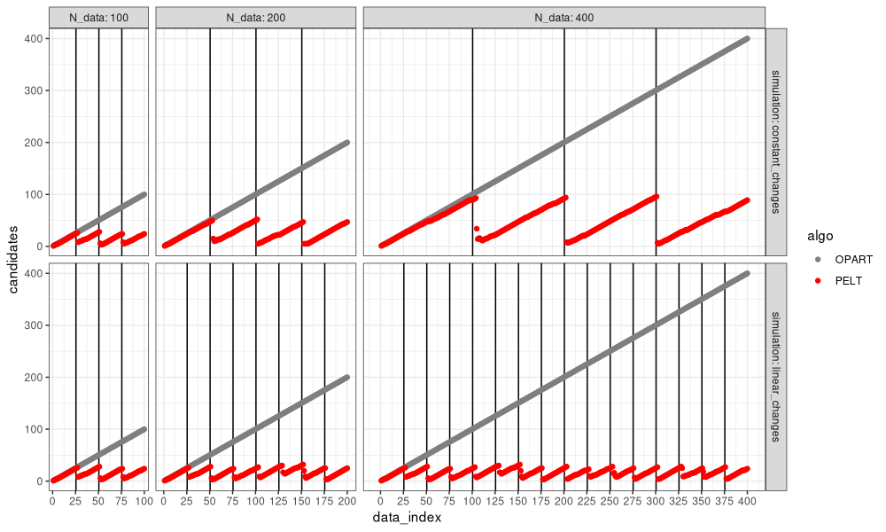
We can see in the figure above that PELT considers a much smaller number of change-points, that tends to reset near zero, for each change-point detected.
- In the bottom simulation with linear changes, the number of change-point candidates considered by PELT is constant (does not depend on number of data), so PELT is linear time, whereas OPART is quadratic, in the number of data.
- In the top simulation with constant changes, the number of change-point candidates considered by PELT is linear in the number of data, so both OPART and PELT are quadratic time in the number of data.
FPOP
Now we run FPOP, which is another pruning method, which is more complex to implement efficiently, so we use C++ code in the R package PeakSegOptimal.
if(FALSE){
  remotes::install_github("tdhock/PeakSegOptimal@f05834ad4b452070da1818f25412e5ac97454833")
}
fpop_info_list <- list()
fpop_segs_list <- list()
for(N_data in N_data_vec){
  for(simulation in names(sim_fun_list)){
    N_sim <- paste(N_data, simulation)
    data_value <- sim_data_list[[N_sim]]$data_value
    pfit <- PeakSegOptimal::UnconstrainedFPOP(
      data_value, penalty=penalty, verbose_file=tempfile())
    both_index_list[[paste(N_data, simulation, "FPOP")]] <- unique(data.table(
      N_data, simulation, algo="FPOP", pfit$index_dt
    )[, let(
      data_index=data_index+1L,
      change=change+2L
    )])
    start <- rev(with(pfit, ends.vec[ends.vec>=0])+1L)
    end <- c(start[-1]-1L,length(data_value))
    fpop_info_list[[paste(N_data,simulation)]] <- data.table(
      N_data,simulation,
      algo="FPOP",
      candidates=pfit$intervals.vec,
      data_index=seq_along(data_value))
    fpop_segs_list[[paste(N_data,simulation)]] <- data.table(
      N_data,simulation,start,end)
  }
}
(fpop_info <- addSim(rbindlist(fpop_info_list)))
##       N_data       simulation   algo candidates data_index         Simulation
##        <num>           <char> <char>      <int>      <int>             <char>
##    1:    100 constant_changes   FPOP          1          1 \nconstant_changes
##    2:    100 constant_changes   FPOP          2          2 \nconstant_changes
##    3:    100 constant_changes   FPOP          3          3 \nconstant_changes
##    4:    100 constant_changes   FPOP          3          4 \nconstant_changes
##    5:    100 constant_changes   FPOP          3          5 \nconstant_changes
##   ---
## 1396:    400   linear_changes   FPOP          5        396   \nlinear_changes
## 1397:    400   linear_changes   FPOP          5        397   \nlinear_changes
## 1398:    400   linear_changes   FPOP          6        398   \nlinear_changes
## 1399:    400   linear_changes   FPOP          6        399   \nlinear_changes
## 1400:    400   linear_changes   FPOP          6        400   \nlinear_changes
(fpop_segs <- rbindlist(fpop_segs_list))
##     N_data       simulation start   end
##      <num>           <char> <int> <int>
##  1:    100 constant_changes    26    50
##  2:    100 constant_changes    51    75
##  3:    100 constant_changes    76   100
##  4:    100 constant_changes   101   100
##  5:    100   linear_changes    26    50
##  6:    100   linear_changes    51    75
##  7:    100   linear_changes    76   100
##  8:    100   linear_changes   101   100
##  9:    200 constant_changes    51   100
## 10:    200 constant_changes   101   150
## 11:    200 constant_changes   151   200
## 12:    200 constant_changes   201   200
## 13:    200   linear_changes    26    50
## 14:    200   linear_changes    51    75
## 15:    200   linear_changes    76   100
## 16:    200   linear_changes   101   125
## 17:    200   linear_changes   126   150
## 18:    200   linear_changes   151   175
## 19:    200   linear_changes   176   200
## 20:    200   linear_changes   201   200
## 21:    400 constant_changes   101   200
## 22:    400 constant_changes   201   300
## 23:    400 constant_changes   301   400
## 24:    400 constant_changes   401   400
## 25:    400   linear_changes    26    50
## 26:    400   linear_changes    51    75
## 27:    400   linear_changes    76   100
## 28:    400   linear_changes   101   125
## 29:    400   linear_changes   126   150
## 30:    400   linear_changes   151   175
## 31:    400   linear_changes   176   201
## 32:    400   linear_changes   202   224
## 33:    400   linear_changes   225   250
## 34:    400   linear_changes   251   275
## 35:    400   linear_changes   276   300
## 36:    400   linear_changes   301   325
## 37:    400   linear_changes   326   350
## 38:    400   linear_changes   351   375
## 39:    400   linear_changes   376   400
## 40:    400   linear_changes   401   400
##     N_data       simulation start   end
both_info <- rbind(pelt_info, fpop_info)
ggplot()+
  theme_bw()+
  theme(
    panel.spacing=grid::unit(1,"lines"),
    text=element_text(size=15))+
  geom_vline(aes(
    xintercept=end+0.5),
    data=sim_changes)+
  scale_color_manual(
    breaks=names(algo.colors),
    values=algo.colors)+
  geom_point(aes(
    data_index, candidates, color=algo),
    data=both_info)+
  facet_grid(Simulation ~ N_data, labeller=label_both, scales="free_x", space="free")+
  scale_x_continuous(
    breaks=seq(0,max(N_data_vec),by=50))
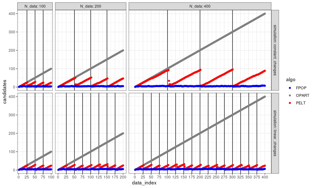
In the figure above, we can see the advantage of FPOP: the number of change-points considered does not increase with the number of data, even with constant number of changes (larger segments).
- In the top simulation with constant changes, the number of change-points candidates considered is linear in the number of data, so both OPART and PELT are quadratic time in the number of data, whereas FPOP is sub-quadratic (empirically linear or log-linear).
DuST
DuST is a new pruning technique based on Lagrange duality, proposed by Truong and Runge, Stat, 2024.
if(FALSE){
  remotes::install_github("vrunge/dust@910f8c67f99354fdb5ff7740e6436eb487d9efa6")
}
set.seed(1)
ex_data <- rpois(7,100)
ex_penalty <- 1
dfit <- dust::dust.1D(ex_data,ex_penalty,"poisson")
rbind(
  PELT=PELT(ex_data,ex_penalty)$cost[-1]/seq_along(ex_data),
  FPOP=PeakSegOptimal::UnconstrainedFPOP(ex_data,penalty=ex_penalty)$cost,
  DUST=dfit$costQ/seq_along(ex_data))
##           [,1]      [,2]      [,3]      [,4]     [,5]      [,6]      [,7]
## PELT -328.5318 -374.3771 -388.3987 -385.9978 -366.236 -368.2061 -371.7383
## FPOP -328.5318 -374.3771 -388.3987 -385.9978 -366.236 -368.2061 -371.7383
## DUST -328.5318 -374.3771 -388.3987 -385.9978 -366.236 -368.2061 -371.7383
The code above verifies that we compute the cost in the same way for each algorithm. In particular, PELT and DUST return the total cost, so we need to divide by the number of data points to get the average cost, which is returned by FPOP. Below we compute the candidates considered by DUST, for each of the two simulations, and a variety of data sizes.
dust_info_list <- list()
dust_segs_list <- list()
for(N_data in N_data_vec){
  for(simulation in names(sim_fun_list)){
    N_sim <- paste(N_data, simulation)
    data_value <- sim_data_list[[N_sim]]$data_value
    dfit <- dust::dust.object.1D("poisson")
    candidates <- rep(NA_integer_, N_data)
    for(data_index in seq_along(data_value)){
      dfit$append_c(data_value[[data_index]], penalty)
      dfit$update_partition()
      pinfo <- dfit$get_partition()
      change <- pinfo$lastIndexSet[-1]+1L
      candidates[[data_index]] <- length(change)
      mean_cost <- pinfo$costQ/seq_along(pinfo$costQ)
      both_index_list[[paste(
        N_data, simulation, "DUST", data_index
      )]] <- data.table(
        N_data, simulation, algo="DUST", data_index,
        change, cost=mean_cost[change])
    }
    end <- pinfo$changepoints
    start <- c(1, end[-length(end)]+1)
    dust_info_list[[paste(N_data,simulation)]] <- data.table(
      N_data,simulation,
      algo="DUST",
      candidates,
      data_index=seq_along(data_value))
    dust_segs_list[[paste(N_data,simulation)]] <- data.table(
      N_data,simulation,start,end)
  }
}
(dust_info <- addSim(rbindlist(dust_info_list)))
##       N_data       simulation   algo candidates data_index         Simulation
##        <num>           <char> <char>      <int>      <int>             <char>
##    1:    100 constant_changes   DUST          1          1 \nconstant_changes
##    2:    100 constant_changes   DUST          1          2 \nconstant_changes
##    3:    100 constant_changes   DUST          1          3 \nconstant_changes
##    4:    100 constant_changes   DUST          1          4 \nconstant_changes
##    5:    100 constant_changes   DUST          2          5 \nconstant_changes
##   ---
## 1396:    400   linear_changes   DUST          4        396   \nlinear_changes
## 1397:    400   linear_changes   DUST          5        397   \nlinear_changes
## 1398:    400   linear_changes   DUST          5        398   \nlinear_changes
## 1399:    400   linear_changes   DUST          5        399   \nlinear_changes
## 1400:    400   linear_changes   DUST          5        400   \nlinear_changes
(dust_segs <- rbindlist(dust_segs_list))
##     N_data       simulation start   end
##      <num>           <char> <num> <num>
##  1:    100 constant_changes     1    25
##  2:    100 constant_changes    26    50
##  3:    100 constant_changes    51    75
##  4:    100 constant_changes    76   100
##  5:    100   linear_changes     1    25
##  6:    100   linear_changes    26    50
##  7:    100   linear_changes    51    75
##  8:    100   linear_changes    76   100
##  9:    200 constant_changes     1    50
## 10:    200 constant_changes    51   100
## 11:    200 constant_changes   101   150
## 12:    200 constant_changes   151   200
## 13:    200   linear_changes     1    25
## 14:    200   linear_changes    26    50
## 15:    200   linear_changes    51    75
## 16:    200   linear_changes    76   100
## 17:    200   linear_changes   101   125
## 18:    200   linear_changes   126   150
## 19:    200   linear_changes   151   175
## 20:    200   linear_changes   176   200
## 21:    400 constant_changes     1   100
## 22:    400 constant_changes   101   200
## 23:    400 constant_changes   201   300
## 24:    400 constant_changes   301   400
## 25:    400   linear_changes     1    25
## 26:    400   linear_changes    26    50
## 27:    400   linear_changes    51    75
## 28:    400   linear_changes    76   100
## 29:    400   linear_changes   101   125
## 30:    400   linear_changes   126   150
## 31:    400   linear_changes   151   175
## 32:    400   linear_changes   176   201
## 33:    400   linear_changes   202   224
## 34:    400   linear_changes   225   250
## 35:    400   linear_changes   251   275
## 36:    400   linear_changes   276   300
## 37:    400   linear_changes   301   325
## 38:    400   linear_changes   326   350
## 39:    400   linear_changes   351   375
## 40:    400   linear_changes   376   400
##     N_data       simulation start   end
three_info <- rbind(pelt_info, fpop_info, dust_info)
ggplot()+
  theme_bw()+
  theme(
    panel.spacing=grid::unit(1,"lines"),
    text=element_text(size=15))+
  geom_vline(aes(
    xintercept=end+0.5),
    data=sim_changes)+
  scale_color_manual(
    breaks=names(algo.colors),
    values=algo.colors)+
  geom_point(aes(
    data_index, candidates, color=algo),
    data=three_info)+
  facet_grid(Simulation ~ N_data, labeller=label_both, scales="free_x", space="free")+
  scale_x_continuous(
    breaks=seq(0,max(N_data_vec),by=50))
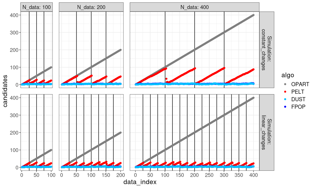
The figure above shows that DUST pruned much more than PELT, nearly the same amount as FPOP.
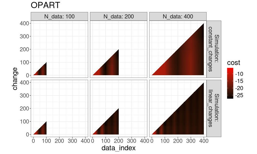
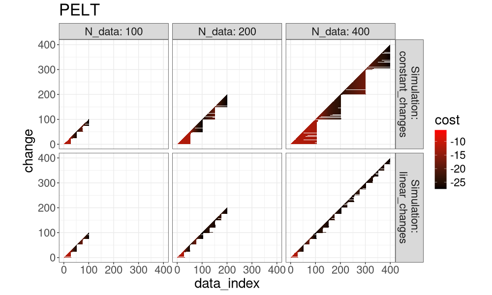
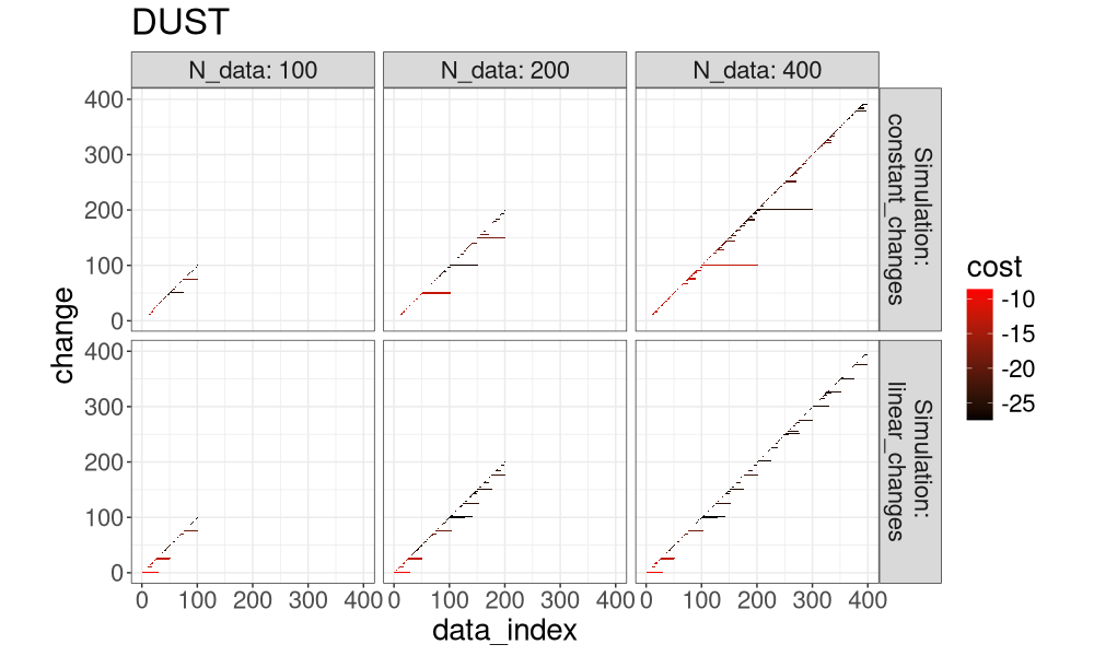
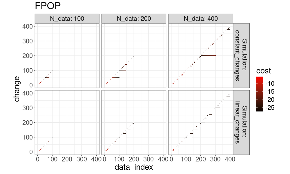
Heat maps
Another way to view this is by looking at the cost of each candidate change-point considered, as in the heat map below.
algo.levs <- c("OPART","PELT","FPOP")
algo.levs <- names(algo.colors)
(both_index <- addSim(rbindlist(both_index_list))[, let(
  Algorithm = factor(algo, algo.levs)
)][])
##         N_data       simulation   algo data_index change       cost         Simulation Algorithm
##          <num>           <char> <char>      <int>  <num>      <num>             <char>    <fctr>
##      1:    100 constant_changes  OPART          1      1  -8.635532 \nconstant_changes     OPART
##      2:    100 constant_changes  OPART          2      1 -10.775021 \nconstant_changes     OPART
##      3:    100 constant_changes  OPART          2      2  -5.830692 \nconstant_changes     OPART
##      4:    100 constant_changes  OPART          3      1  -9.335529 \nconstant_changes     OPART
##      5:    100 constant_changes  OPART          3      2  -6.005552 \nconstant_changes     OPART
##     ---
## 257086:    400   linear_changes   DUST        400    397 -26.828554   \nlinear_changes      DUST
## 257087:    400   linear_changes   DUST        400    395 -26.734206   \nlinear_changes      DUST
## 257088:    400   linear_changes   DUST        400    394 -26.703759   \nlinear_changes      DUST
## 257089:    400   linear_changes   DUST        400    393 -26.639462   \nlinear_changes      DUST
## 257090:    400   linear_changes   DUST        400    376 -24.830653   \nlinear_changes      DUST
both_index[data_index==2 & N_data==400 & simulation=="constant_changes"]
##    N_data       simulation   algo data_index change       cost         Simulation Algorithm
##     <num>           <char> <char>      <int>  <num>      <num>             <char>    <fctr>
## 1:    400 constant_changes  OPART          2      1 -10.775021 \nconstant_changes     OPART
## 2:    400 constant_changes  OPART          2      2  -5.830692 \nconstant_changes     OPART
## 3:    400 constant_changes   PELT          2      1 -10.775021 \nconstant_changes      PELT
## 4:    400 constant_changes   PELT          2      2  -5.830692 \nconstant_changes      PELT
## 5:    400 constant_changes   FPOP          2      2  -5.830690 \nconstant_changes      FPOP
## 6:    400 constant_changes   FPOP          2      1 -10.775000 \nconstant_changes      FPOP
## 7:    400 constant_changes   DUST          2      1  -8.635532 \nconstant_changes      DUST
for(a in algo.levs){
  gg <- ggplot()+
    ggtitle(a)+
    theme_bw()+
    theme(text=element_text(size=20))+
    coord_equal()+
    geom_tile(aes(
      data_index, change, fill=cost),
      data=both_index[Algorithm==a])+
    scale_fill_gradient(low="black", high="red")+
    facet_grid(Simulation ~ N_data, label=label_both)
  print(gg)
}
Another way to visualize it is in the plot below, which super-imposes the three algos.
ggplot()+
  theme_bw()+
  theme(text=element_text(size=15))+
  geom_tile(aes(
    data_index, change, fill=Algorithm),
    data=both_index)+
  scale_fill_manual(values=algo.colors)+
  scale_x_continuous(
    breaks=seq(0,max(N_data_vec),by=50))+
  facet_grid(Simulation ~ N_data, label=label_both, scales="free", space="free")
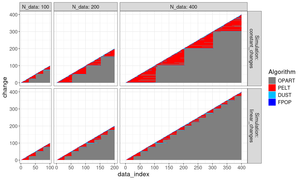
It is clear that FPOP prunes much more than PELT, especially in the case of constant changes (segments that get larger with the overall number of data). It is also clear that DUST considers nearly the same change-points as FPOP.
atime comparison
The atime() function can be used to perform asymptotic time/memory/etc comparisons.
This means that we will increase N, and monitor how fast certain quantities grow with N.
We begin by defining the data sizes N of interest:
base_N <- c(100,200,400,800)
(all_N <- unlist(lapply(10^seq(0,4), function(x)x*base_N)))
##  [1] 1e+02 2e+02 4e+02 8e+02 1e+03 2e+03 4e+03 8e+03 1e+04 2e+04 4e+04 8e+04 1e+05 2e+05 4e+05 8e+05 1e+06 2e+06 4e+06
## [20] 8e+06
The data sizes above are on a log scale between 10 and 1,000,000. Next, we define a list that enumerates the different combinations in the experiment.
grid_args <- list(
  list(simulation=names(sim_fun_list)),
  DUST=quote({
    dfit <- dust::dust.1D(data_list[[simulation]], penalty, "poisson")
    with(dfit, data.frame(
      mean_candidates=mean(nb),
      segments=length(changepoints),
      max_seg_size=max(diff(c(0,changepoints)))))
  }),
  FPOP=quote({
    pfit <- PeakSegOptimal::UnconstrainedFPOP(
      data_list[[simulation]], penalty=penalty)
    data.frame(
      mean_candidates=mean(pfit$intervals.vec),
      segments=sum(is.finite(pfit$mean.vec)),
      max_seg_size=max(-diff(pfit$ends.vec)))
  }))
for(algo in names(algo.prune)){
  prune <- algo.prune[[algo]]
  grid_args[[algo]] <- substitute({
    fit <- PELT(data_list[[simulation]], penalty=penalty, prune=prune)
    dec <- decode(fit$change)
    data.frame(
      mean_candidates=mean(fit$candidates),
      segments=nrow(dec),
      max_seg_size=max(diff(c(0,dec$last.i))))
  }, list(prune=prune))
}
(expr.list <- do.call(atime::atime_grid, grid_args))
## $`DUST simulation=constant_changes`
## {
##     dfit <- dust::dust.1D(data_list[["constant_changes"]], penalty,
##         "poisson")
##     with(dfit, data.frame(mean_candidates = mean(nb), segments = length(changepoints),
##         max_seg_size = max(diff(c(0, changepoints)))))
## }
##
## $`DUST simulation=linear_changes`
## {
##     dfit <- dust::dust.1D(data_list[["linear_changes"]], penalty,
##         "poisson")
##     with(dfit, data.frame(mean_candidates = mean(nb), segments = length(changepoints),
##         max_seg_size = max(diff(c(0, changepoints)))))
## }
##
## $`FPOP simulation=constant_changes`
## {
##     pfit <- PeakSegOptimal::UnconstrainedFPOP(data_list[["constant_changes"]],
##         penalty = penalty)
##     data.frame(mean_candidates = mean(pfit$intervals.vec), segments = sum(is.finite(pfit$mean.vec)),
##         max_seg_size = max(-diff(pfit$ends.vec)))
## }
##
## $`FPOP simulation=linear_changes`
## {
##     pfit <- PeakSegOptimal::UnconstrainedFPOP(data_list[["linear_changes"]],
##         penalty = penalty)
##     data.frame(mean_candidates = mean(pfit$intervals.vec), segments = sum(is.finite(pfit$mean.vec)),
##         max_seg_size = max(-diff(pfit$ends.vec)))
## }
##
## $`OPART simulation=constant_changes`
## {
##     fit <- PELT(data_list[["constant_changes"]], penalty = penalty,
##         prune = FALSE)
##     dec <- decode(fit$change)
##     data.frame(mean_candidates = mean(fit$candidates), segments = nrow(dec),
##         max_seg_size = max(diff(c(0, dec$last.i))))
## }
##
## $`OPART simulation=linear_changes`
## {
##     fit <- PELT(data_list[["linear_changes"]], penalty = penalty,
##         prune = FALSE)
##     dec <- decode(fit$change)
##     data.frame(mean_candidates = mean(fit$candidates), segments = nrow(dec),
##         max_seg_size = max(diff(c(0, dec$last.i))))
## }
##
## $`PELT simulation=constant_changes`
## {
##     fit <- PELT(data_list[["constant_changes"]], penalty = penalty,
##         prune = TRUE)
##     dec <- decode(fit$change)
##     data.frame(mean_candidates = mean(fit$candidates), segments = nrow(dec),
##         max_seg_size = max(diff(c(0, dec$last.i))))
## }
##
## $`PELT simulation=linear_changes`
## {
##     fit <- PELT(data_list[["linear_changes"]], penalty = penalty,
##         prune = TRUE)
##     dec <- decode(fit$change)
##     data.frame(mean_candidates = mean(fit$candidates), segments = nrow(dec),
##         max_seg_size = max(diff(c(0, dec$last.i))))
## }
##
## attr(,"parameters")
##                            expr.name expr.grid       simulation
##                               <char>    <char>           <char>
## 1:  DUST simulation=constant_changes      DUST constant_changes
## 2:    DUST simulation=linear_changes      DUST   linear_changes
## 3:  FPOP simulation=constant_changes      FPOP constant_changes
## 4:    FPOP simulation=linear_changes      FPOP   linear_changes
## 5: OPART simulation=constant_changes     OPART constant_changes
## 6:   OPART simulation=linear_changes     OPART   linear_changes
## 7:  PELT simulation=constant_changes      PELT constant_changes
## 8:    PELT simulation=linear_changes      PELT   linear_changes
Above we see a list with 8 expressions to run, and a data table with the corresponding number of rows. Note that each expression
- returns a data frame with one row and three columns that will be used as units to analyze as a function of N.
- should depend on data size N, which does not appear in the
expressions above, but it is used to define
data_listin thesetupargument below:
cache.rds <- "2025-02-25-PELT-vs-FPOP.rds"
if(file.exists(cache.rds)){
  atime_list <- readRDS(cache.rds)
}else{
  atime_list <- atime::atime(
    N=all_N,
    setup={
      data_list <- list()
      for(simulation in names(sim_fun_list)){
        sim_fun <- sim_fun_list[[simulation]]
        data_mean_vec <- sim_fun(N)
        set.seed(1)
        data_list[[simulation]] <- rpois(N, data_mean_vec)
      }
    },
    expr.list=expr.list,
    seconds.limit=1,
    result=TRUE)
  saveRDS(atime_list, cache.rds)
}
Note in the code above that we run the timing inside if(file.exists, which is a caching mechanism.
The result is time-consuming to compute, so the first time it is computed, it is saved to disk as an RDS file, and then subsequently read from disk, to save time.
Finally, we plot the different units as a function of data size N, in the figure below.
refs_list <- atime::references_best(atime_list)
ggplot()+
  theme(
    axis.text.x=element_text(size=12,angle=30,hjust=1),
    text=element_text(size=12))+
  directlabels::geom_dl(aes(
    N, empirical, color=expr.grid, label=expr.grid),
    data=refs_list$measurements,
    method="right.polygons")+
  geom_line(aes(
    N, empirical, color=expr.grid),
    data=refs_list$measurements)+
  scale_color_manual(
    "algorithm",
    guide="none",
    values=algo.colors)+
  facet_grid(unit ~ simulation, scales="free")+
  scale_x_log10(
    "N = number of data in sequence",
    breaks=10^seq(2,7),
    limits=c(NA, 1e8))+
  scale_y_log10("")
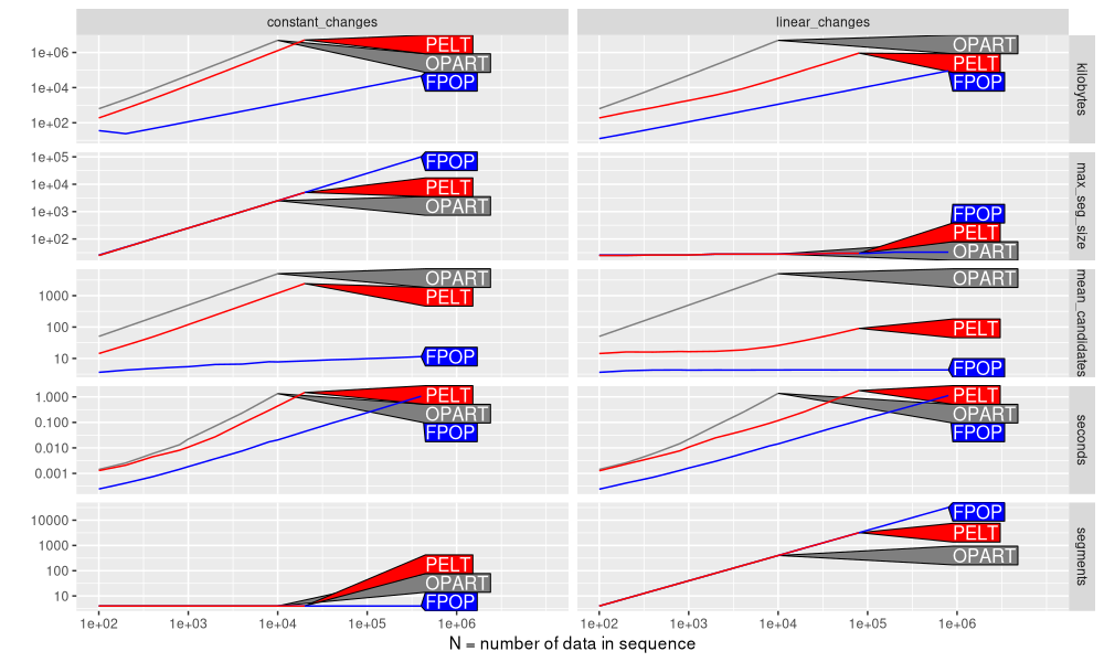
Above the figure shows a different curve for each algorithm, and a different panel for each simulation and measurement unit. We can observe that
- PELT memory usage in kilobytes has a larger slope for constant changes, than for linear changes. This implies a larger asymptotic complexity class.
- The maximum segment size,
max_seg_size, is the same for all algos, indicating that the penalty was chosen appropriately, and the algorithms are computing the same optimal solution. - Similarly, the mean number of candidates considered by the PELT algorithm has a larger slope for constant changes (same as OPART/linear in N), than for linear changes (relatively constant).
- For PELT seconds, we see a slightly larger slope for seconds in constant changes, compared to linear changes.
- As expected, number of
segmentsis constant for a constant number of changes (left), and increasing for a linear number of changes (right).
Below we plot the same data in a different way, that facilitates comparisons across the type of simulation:
refs_list$meas[, let(
  Simulation = sub("_","\n",simulation),
  Algorithm = factor(expr.grid, algo.levs)
)][]
##              unit                         expr.name fun.name fun.latex expr.grid       simulation     N          min
##            <char>                            <char>   <char>    <char>    <char>           <char> <num>        <num>
##   1:    kilobytes  DUST simulation=constant_changes        N         N      DUST constant_changes 1e+02 0.0003783300
##   2:    kilobytes    DUST simulation=linear_changes        N         N      DUST   linear_changes 1e+02 0.0003679921
##   3:    kilobytes  FPOP simulation=constant_changes        N         N      FPOP constant_changes 1e+02 0.0002385300
##   4:    kilobytes    FPOP simulation=linear_changes        N         N      FPOP   linear_changes 1e+02 0.0002388670
##   5:    kilobytes OPART simulation=constant_changes      N^2       N^2     OPART constant_changes 1e+02 0.0017725271
##  ---
## 531: max_seg_size    DUST simulation=linear_changes     <NA>      <NA>      DUST   linear_changes 1e+06 0.2073926179
## 532: max_seg_size  DUST simulation=constant_changes        N         N      DUST constant_changes 2e+06 1.2038735760
## 533: max_seg_size    DUST simulation=linear_changes     <NA>      <NA>      DUST   linear_changes 2e+06 0.4109501251
## 534: max_seg_size    DUST simulation=linear_changes     <NA>      <NA>      DUST   linear_changes 4e+06 0.8158070830
## 535: max_seg_size    DUST simulation=linear_changes     <NA>      <NA>      DUST   linear_changes 8e+06 1.7653503710
##            median      itr/sec    gc/sec n_itr  n_gc            result                                        time
##             <num>        <num>     <num> <int> <num>            <list>                                      <list>
##   1: 0.0004352505 2154.4517374 0.0000000    10     0 <data.frame[1x3]>     684µs,461µs,559µs,460µs,443µs,428µs,...
##   2: 0.0004020535 2401.6036997 0.0000000    10     0 <data.frame[1x3]>     539µs,440µs,376µs,375µs,368µs,368µs,...
##   3: 0.0002547929 3821.8312727 0.0000000    10     0 <data.frame[1x3]>     352µs,266µs,253µs,257µs,244µs,239µs,...
##   4: 0.0002549275 3717.6576328 0.0000000    10     0 <data.frame[1x3]>     330µs,259µs,245µs,251µs,244µs,260µs,...
##   5: 0.0018963466  512.9685126 0.0000000    10     0 <data.frame[1x3]> 2.22ms,1.95ms,1.9ms,2.25ms,1.88ms,1.8ms,...
##  ---
## 531: 0.2092330895    4.7958287 2.0553552     7     3 <data.frame[1x3]>     215ms,207ms,208ms,208ms,211ms,210ms,...
## 532: 1.2085569665    0.8285637 0.5523758     6     4 <data.frame[1x3]>      1.21s,1.2s,1.21s,1.21s,1.22s,1.21s,...
## 533: 0.4198099815    2.3654731 2.8385677     5     6 <data.frame[1x3]>     411ms,421ms,412ms,413ms,413ms,428ms,...
## 534: 0.8427591324    1.1720689 5.8603445     2    10 <data.frame[1x3]>     891ms,908ms,944ms,816ms,842ms,835ms,...
## 535: 1.8154073436    0.5504069 1.0457731    10    19 <data.frame[1x3]>     1.85s,1.77s,1.88s,1.77s,1.77s,1.76s,...
##                  gc    kilobytes          q25          q75          max         mean           sd mean_candidates
##              <list>        <num>        <num>        <num>        <num>        <num>        <num>           <num>
##   1: <tbl_df[10x3]> 2.771094e+01 0.0004209292 0.0004610748 0.0006840620 0.0004641552 9.201532e-05        2.670000
##   2: <tbl_df[10x3]> 4.414062e+00 0.0003704191 0.0004380470 0.0005388900 0.0004163884 5.674954e-05        2.670000
##   3: <tbl_df[10x3]> 1.260156e+01 0.0002417532 0.0002634847 0.0003524380 0.0002616547 3.369264e-05        3.620000
##   4: <tbl_df[10x3]> 1.260156e+01 0.0002441385 0.0002641595 0.0003569479 0.0002689866 4.085838e-05        3.620000
##   5: <tbl_df[10x3]> 8.858906e+02 0.0018204999 0.0020173791 0.0022495311 0.0019494374 1.699584e-04       50.500000
##  ---
## 531: <tbl_df[10x3]> 4.156473e+04 0.2079193987 0.2104281450 0.2152205879 0.2098437335 2.562125e-03        3.217038
## 532: <tbl_df[10x3]> 7.812627e+04 1.2058141263 1.2152456919 1.2191310481 1.2103568259 5.685315e-03       17.992054
## 533: <tbl_df[10x3]> 8.312638e+04 0.4129259010 0.4416093705 0.4589046910 0.4271669130 1.776231e-02        3.215730
## 534: <tbl_df[10x3]> 1.662524e+05 0.8338015667 0.8974753255 0.9439399519 0.8642597747 4.272027e-02        3.213032
## 535: <tbl_df[10x3]> 3.325031e+05 1.7716509304 1.8610300747 1.8748299400 1.8168377176 4.841334e-02        3.212893
##      segments max_seg_size                             expr.class                                  expr.latex
##         <int>        <num>                                 <char>                                      <char>
##   1:        4           25    DUST simulation=constant_changes\nN    DUST simulation=constant_changes\n$O(N)$
##   2:        4           25      DUST simulation=linear_changes\nN      DUST simulation=linear_changes\n$O(N)$
##   3:        4           26    FPOP simulation=constant_changes\nN    FPOP simulation=constant_changes\n$O(N)$
##   4:        4           26      FPOP simulation=linear_changes\nN      FPOP simulation=linear_changes\n$O(N)$
##   5:        4           25 OPART simulation=constant_changes\nN^2 OPART simulation=constant_changes\n$O(N^2)$
##  ---
## 531:    40003           33     DUST simulation=linear_changes\nNA     DUST simulation=linear_changes\n$O(NA)$
## 532:        4       500000    DUST simulation=constant_changes\nN    DUST simulation=constant_changes\n$O(N)$
## 533:    80005           34     DUST simulation=linear_changes\nNA     DUST simulation=linear_changes\n$O(NA)$
## 534:   160014           34     DUST simulation=linear_changes\nNA     DUST simulation=linear_changes\n$O(NA)$
## 535:   320033           38     DUST simulation=linear_changes\nNA     DUST simulation=linear_changes\n$O(NA)$
##         empirical        Simulation Algorithm
##             <num>            <char>    <fctr>
##   1: 2.771094e+01 constant\nchanges      DUST
##   2: 4.414062e+00   linear\nchanges      DUST
##   3: 1.260156e+01 constant\nchanges      FPOP
##   4: 1.260156e+01   linear\nchanges      FPOP
##   5: 8.858906e+02 constant\nchanges     OPART
##  ---
## 531: 3.300000e+01   linear\nchanges      DUST
## 532: 5.000000e+05 constant\nchanges      DUST
## 533: 3.400000e+01   linear\nchanges      DUST
## 534: 3.400000e+01   linear\nchanges      DUST
## 535: 3.800000e+01   linear\nchanges      DUST
ggplot()+
  theme(
    axis.text.x=element_text(size=12,angle=30,hjust=1),
    legend.position="none",
    text=element_text(size=12))+
  directlabels::geom_dl(aes(
    N, empirical, color=Simulation, label=Simulation),
    data=refs_list$measurements,
    method="right.polygons")+
  geom_line(aes(
    N, empirical, color=Simulation),
    data=refs_list$measurements)+
  facet_grid(unit ~ Algorithm, scales="free")+
  scale_x_log10(
    "N = number of data in sequence",
    breaks=10^seq(2,7),
    limits=c(NA, 1e8))+
  scale_y_log10("")
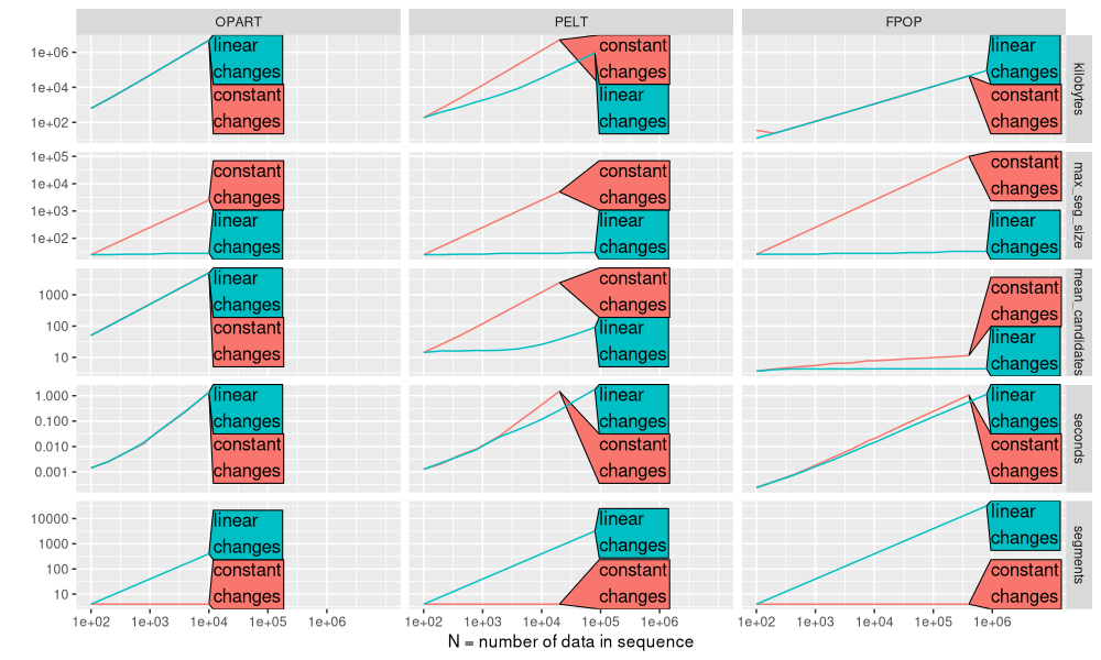
The plot above makes it easier to notice some interesting trends in the mean number of candidates:
- For PELT and FPOP the mean number of candidates is increases for a constant number of changes, but at different rates (FPOP much slower than PELT).
expr.levs <- CJ(
  algo=algo.levs,
  simulation=names(sim_fun_list)
)[algo.levs, paste0(algo,"\n",simulation), on="algo"]
edit_expr <- function(DT)DT[
, expr.name := factor(sub(" simulation=", "\n", expr.name), expr.levs)]
edit_expr(refs_list$meas)
edit_expr(refs_list$plot.ref)
plot(refs_list)+
  theme(
    axis.text.x=element_text(angle=30,hjust=1),
    panel.spacing=grid::unit(1,"lines"))
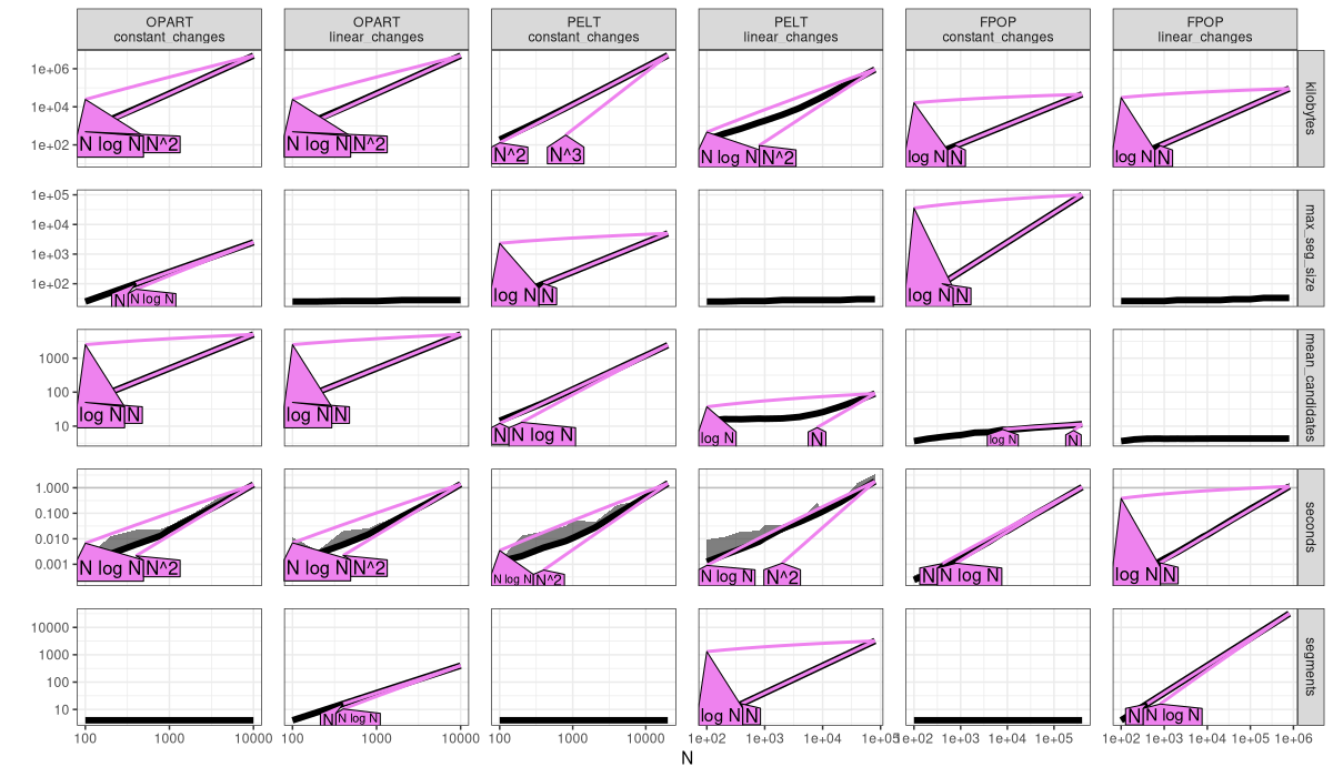
The plot above is an empirical verification of our earlier complexity claims.
- OPART
mean_candidatesis linear,O(N), and time and memory are quadratic,O(N^2). - PELT with constant changes has linear
mean_candidates,O(N), and quadratic time and memory,O(N^2)(same as OPART, no asymptotic speedup). - PELT with linear changes has sub-linear
mean_candidates(constant or log), and linear or log-linear time/memory. - FPOP always has sub-linear
mean_candidates(constant or log), and linear or log-linear time/memory.
The code/plot below shows the speedups in this case.
pred_list <- predict(refs_list)
ggplot()+
  theme_bw()+
  theme(
    text=element_text(size=20))+
  geom_line(aes(
    N, empirical, color=expr.grid),
    data=pred_list$measurements[unit=="seconds"])+
  directlabels::geom_dl(aes(
    N, unit.value, color=expr.grid, label=sprintf(
      "%s\n%s\nN=%s",
      expr.grid,
      ifelse(expr.grid %in% c("FPOP","DUST"), "C++", "R"),
      format(round(N), big.mark=",", scientific=FALSE, trim=TRUE))),
    data=pred_list$prediction,
    method=list(cex=1.5,"top.polygons"))+
  scale_color_manual(
    "algorithm",
    guide="none",
    values=algo.colors)+
  facet_grid(. ~ simulation, scales="free", labeller=label_both)+
  scale_x_log10(
    "N = number of data in sequence",
    breaks=10^seq(2,7),
    limits=c(NA, 1e8))+
  scale_y_log10(
    "Computation time (seconds)",
    breaks=10^seq(-3,0),
    limits=10^c(-4,1))
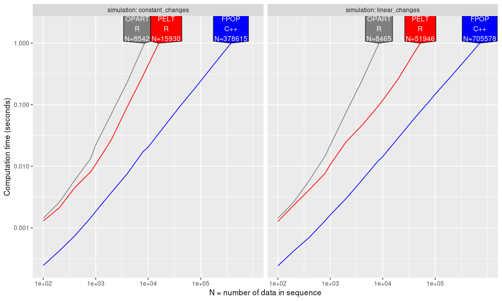
The figure above shows the throughput (data size N) which is possible to compute in 1 second using each algorithm. We see that FPOP is 10-100x faster than OPART/PELT. Part of the difference is that OPART/PELT were coded in R, whereas FPOP was coded in C++ (faster). Another difference is that FPOP is asymptotically faster with constant changes, as can be seen by a smaller slope for FPOP, compared to OPART/PELT.
Below we zoom in on the number of candidate change-points considered by each algorithm.
cand_dt <- pred_list$measurements[unit=="mean_candidates"]
ggplot()+
  theme_bw()+
  theme(
    axis.text.x=element_text(size=20,angle=30,hjust=1),
    text=element_text(size=20))+
  geom_line(aes(
    N, empirical, color=expr.grid),
    data=cand_dt)+
  directlabels::geom_dl(aes(
    N, empirical, color=expr.grid, label=expr.grid),
    data=cand_dt,
    method=list(cex=2, "right.polygons"))+
  scale_color_manual(
    "algorithm",
    guide="none",
    values=algo.colors)+
  facet_grid(. ~ simulation, scales="free", labeller=label_both)+
  scale_x_log10(
    "N = number of data in sequence",
    breaks=10^seq(2,7,by=1),
    limits=c(NA, 5e8))+
  scale_y_log10("Mean number of candidate change-points")
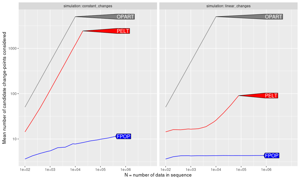
The figure above shows that
- OPART always considers a linear number of candidates (slow).
- PELT also considers a linear number of candidates (slow), when the number of changes is constant.
- PELT considers a sub-linear number of candidates (fast), when the number of changes is linear.
- FPOP always considers sub-linear number of candidates (fast), which is either constant for a linear number of changes, or logarithmic for a constant number of changes.
Conclusions
We have explored three algorithms for optimal change-point detection.
- The classic OPART algorithm is always quadratic time in the number of data to segment.
- The Pruned Exact Linear Time (PELT) algorithm can indeed be linear time in the number of data to segment, but only when the number of change-points grows with the number of data points. When the number of change-points is constant, there are ever-increasing segments, and the PELT algorithm must compute a cost for each candidate on these large segments; in this situation, PELT suffers from the same quadratic time complexity as OPART.
- The FPOP algorithm is fast (linear or log-linear) in both of the scenarios we examined.
We performed the comparison for count data (Poisson loss), but we could do something similar for real data (square loss), by modifying one of these implementations of dynamic programming:
Session info
sessionInfo()
## R version 4.5.0 (2025-04-11)
## Platform: x86_64-pc-linux-gnu
## Running under: Ubuntu 24.04.2 LTS
##
## Matrix products: default
## BLAS:   /usr/lib/x86_64-linux-gnu/blas/libblas.so.3.12.0
## LAPACK: /usr/lib/x86_64-linux-gnu/lapack/liblapack.so.3.12.0  LAPACK version 3.12.0
##
## locale:
##  [1] LC_CTYPE=fr_FR.UTF-8       LC_NUMERIC=C               LC_TIME=fr_FR.UTF-8        LC_COLLATE=fr_FR.UTF-8
##  [5] LC_MONETARY=fr_FR.UTF-8    LC_MESSAGES=fr_FR.UTF-8    LC_PAPER=fr_FR.UTF-8       LC_NAME=C
##  [9] LC_ADDRESS=C               LC_TELEPHONE=C             LC_MEASUREMENT=fr_FR.UTF-8 LC_IDENTIFICATION=C
##
## time zone: Europe/Paris
## tzcode source: system (glibc)
##
## attached base packages:
## [1] stats     graphics  grDevices utils     datasets  methods   base
##
## other attached packages:
## [1] ggplot2_3.5.1     data.table_1.17.0
##
## loaded via a namespace (and not attached):
##  [1] directlabels_2024.1.21   vctrs_0.6.5              cli_3.6.4                knitr_1.50
##  [5] rlang_1.1.5              xfun_0.51                penaltyLearning_2024.9.3 bench_1.1.4
##  [9] generics_0.1.3           glue_1.8.0               labeling_0.4.3           colorspace_2.1-1
## [13] scales_1.3.0             quadprog_1.5-8           grid_4.5.0               munsell_0.5.1
## [17] evaluate_1.0.3           tibble_3.2.1             profmem_0.6.0            lifecycle_1.0.4
## [21] compiler_4.5.0           codetools_0.2-20         dplyr_1.1.4              dust_0.3.0
## [25] Rcpp_1.0.14              pkgconfig_2.0.3          PeakSegOptimal_2025.3.31 atime_2025.4.1
## [29] lattice_0.22-6           farver_2.1.2             R6_2.6.1                 tidyselect_1.2.1
## [33] pillar_1.10.1            magrittr_2.0.3           tools_4.5.0              withr_3.0.2
## [37] gtable_0.3.6             remotes_2.5.0