AUC and AUM in torch
The goal of this post is to show how to use torch to compute ROC-AUC (classic evaluation metric for binary classification) and AUM (Area Under Min of False Positive and False Negative rates, our newly Proposed surrogate loss for ROC curve optimization).
- Paper: Optimizing ROC Curves with a Sort-Based Surrogate Loss for Binary Classification and Changepoint Detection.
- Slides PDF.
Introduction: binary classification and zero-one loss
In supervised binary classification, our goal is to learn a function
f using training inputs/features x, and outputs/labels y, such
that f(x)=y (on new/test data). To illustrate, the code below
defines a data set with four samples:
import torch
four_labels = torch.tensor([-1,-1,1,1])
four_pred = torch.tensor([2.0, -3.5, -1.0, 1.5])
Note that four_pred in the code above is a vector of four f(x)
values (real numbers=predicted scores), and four_labels is a vector
of four y values (-1 for negative class, 1 for positive class). How
do we compute if these are good predictions for these labels?
To answer that question, we use an objective function, which computes a number that determines how good/bad our predictions are, relative to the labels in our data set.
The classic objective function for
evaluation is the zero-one loss, which computes the number/proportion
of labels which are mis-classified (in the test set).
The zero-one loss first each real-valued f(x) score to a class by thresholding at zero, and then computes the proportion of predicted classes that do not match the label classes.
def score_to_class(pred_score):
    return torch.where(pred_score < 0, -1, 1)
def pred_is_correct(pred_score, label_vec):
    pred_class = score_to_class(pred_score)
    return pred_class == label_vec
def zero_one_loss(pred_score, label_vec):
    return torch.where(pred_is_correct(pred_score, label_vec), 0, 1)
import pandas as pd
zero_one_df = pd.DataFrame({
    "label":four_labels,
    "score":four_pred,
    "zero_one_loss":zero_one_loss(four_pred, four_labels)
})
zero_one_df
##    label  score  zero_one_loss
## 0     -1    2.0              1
## 1     -1   -3.5              0
## 2      1   -1.0              1
## 3      1    1.5              0
The output above is a table with one row for each sample. The zero_one_loss column shows that if the sign of the score matches the label, then the zero-one loss is 0 (correct), otherwise it is 1 (incorrect). Below we take the mean of that vector, to get the proportion of incorrectly predicted labels:
zero_one_df.zero_one_loss.mean()
## 0.5
The output above indicates that 50% of the rows are classified incorrectly.
Imbalanced data and confusion matrices
In imbalanced data, for example with 99% negative and 1% positive labels, other objective functions like AUC (Area Under ROC Curve) are used for evaluation. The Receiver Operating Characteristic (ROC) curve is a plot of True Positive Rate, as a function of False Positive Rate. What are those?
- True Positive is when
f(x) > 0(predict positive), andy=1(label positive), this is good! The opposite/negative prediction,f(x) < 0, with the same positive label, is called a False Negative (bad). - False Positive is when
f(x) > 0(predict positive), buty=0(label negative), this is bad! The opposite/positive prediction,f(x) < 0, with the same negative label, is called a True Negative (good).
These terms are also names for the entries in the confusion matrix,
| prediction | ||
|---|---|---|
| label | negative, f(x) < 0 |
positive, f(x) > 0 |
negative, y = -1 |
True Negative | False Positive |
negative, y = 1 |
False Negative | True Positive |
Below we add a confusion column with these names to our previous table:
import numpy as np
def TF_pos_neg(pred_score, label_vec):
    pred_is_positive = score_to_class(pred_score) == 1
    pred_name = np.where(pred_is_positive, "Positive", "Negative")
    T_or_F = pred_is_correct(pred_score, label_vec).numpy()
    T_or_F_space = np.char.add(T_or_F.astype(str), " ")
    return np.char.add(T_or_F_space, pred_name)
zero_one_df["confusion"]=TF_pos_neg(four_pred, four_labels)
zero_one_df
##    label  score  zero_one_loss       confusion
## 0     -1    2.0              1  False Positive
## 1     -1   -3.5              0   True Negative
## 2      1   -1.0              1  False Negative
## 3      1    1.5              0   True Positive
The confusion column shows where each sample would appear in the
confusion matrix. When we compute a ROC curve, we compute two
quantities. First, the True Positive Rate (TPR) is the number of true
positives, divided by the number of possible true positives (number of
positive labels).
def get_TPR(df):
    return (df.confusion=="True Positive").sum()/(df.label==1).sum()
get_TPR(zero_one_df)
## 0.5
Next, the False Positive Rate (FPR) is the number of false positives, divided by the number of possible false positives (number of negative labels).
def get_FPR(df):
    return (df.confusion=="False Positive").sum()/(df.label== -1).sum()
get_FPR(zero_one_df)
## 0.5
Both True Positive Rate and False Positive Rate are 0.5 in this example, because there are two of each label; one of each label is mis-classified.
ROC curve computation
When we compute a ROC curve, we need to consider all possible
thresholds of the predicted score f(x), not just the default
threshold of zero. In other words, the ROC curve is a 2D parametric
function: [FPR(c),TPR(c)], where the parameter is c, a constant
that could be added to predicted scores, before using the threshold of
zero to determine whether we should predict if the class is positive
(f(x)+c > 0) or negative (f(x)+c < 0).
If c is very large, then f(x_i)+c > 0 for all data i, so
FPR(c)=1 and TPR(c)=1 (all data classified as positive as in the
code below).
def error_one_constant(constant):
    pred_const = four_pred+constant
    return pd.DataFrame({
        "label":four_labels,
        "score":four_pred,
        "score_plus_constant":pred_const,
        "zero_one_loss":zero_one_loss(pred_const, four_labels),
        "confusion":TF_pos_neg(pred_const, four_labels)
    })
error_one_constant(5)
##    label  score  score_plus_constant  zero_one_loss       confusion
## 0     -1    2.0                  7.0              1  False Positive
## 1     -1   -3.5                  1.5              1  False Positive
## 2      1   -1.0                  4.0              0   True Positive
## 3      1    1.5                  6.5              0   True Positive
If c is very small, then f(x_i)+c < 0 for all data i, so
FPR(c)=0 and TPR(c)=0 (all data classified as negative as in the code below).
error_one_constant(-10)
##    label  score  score_plus_constant  zero_one_loss       confusion
## 0     -1    2.0                 -8.0              0   True Negative
## 1     -1   -3.5                -13.5              0   True Negative
## 2      1   -1.0                -11.0              1  False Negative
## 3      1    1.5                 -8.5              1  False Negative
Note that there are infinitely many different constants which we could add to the predicted values, which result in the same confusion values, and therefore the same point on the ROC curve. For example, below is another small constant which results in all negative predictions:
error_one_constant(-20)
##    label  score  score_plus_constant  zero_one_loss       confusion
## 0     -1    2.0                -18.0              0   True Negative
## 1     -1   -3.5                -23.5              0   True Negative
## 2      1   -1.0                -21.0              1  False Negative
## 3      1    1.5                -18.5              1  False Negative
We can compute a ROC curve (inefficiently, quadratic time in the number of samples) by looping over constants, and repeating the computations, as in the code below.
four_roc_df_list = []
constant_vec = list(-four_pred)+[-torch.inf]
constant_vec.sort()
def one_roc_point(constant):
    one_df = error_one_constant(constant)
    return pd.DataFrame({
        "constant":[float(constant)],
        "TPR":get_TPR(one_df),
        "FPR":get_FPR(one_df)
    })
roc_inefficient_df = pd.concat([
    one_roc_point(constant) for constant in constant_vec
])
roc_inefficient_df
##    constant  TPR  FPR
## 0      -inf  0.0  0.0
## 0      -2.0  0.0  0.5
## 0      -1.5  0.5  0.5
## 0       1.0  1.0  0.5
## 0       3.5  1.0  1.0
The table above has one row for each point on the ROC curve, which is visualized using the code below.
import plotnine as p9
p9.options.figure_size=(8,4)#https://github.com/rstudio/reticulate/issues/1140
gg_roc_inefficient = p9.ggplot()+\
    p9.theme(figure_size=(4,4))+\
    p9.coord_equal()+\
    p9.geom_line(
        p9.aes(
            x="FPR",
            y="TPR",
        ),
        data=roc_inefficient_df
    )+\
    p9.geom_point(
        p9.aes(
            x="FPR",
            y="TPR",
        ),
        data=roc_inefficient_df
    )
show("gg_roc_inefficient")
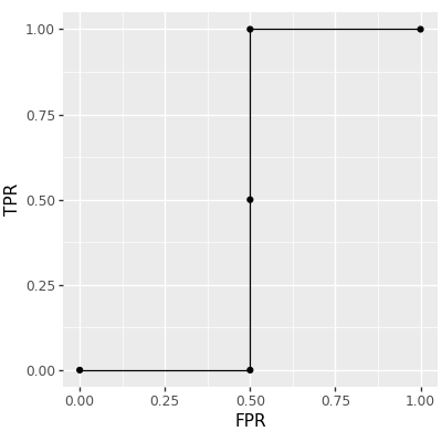
The figure above shows a ROC curve with 5 points (the maximum number of points for 4 data; there could be fewer if there are ties in the predicted scores vector). We mentioned above that it was computed inefficiently, which is caused by the for loop over constants. To avoid that loop (quadratic time overall), we can instead sort the predicted scores (log-linear time overall), and use the cumulative sum, as in the code below:
def ROC_curve(pred_tensor, label_tensor):
    """Receiver Operating Characteristic curve.
    """
    is_positive = label_tensor == 1
    is_negative = label_tensor != 1
    fn_diff = torch.where(is_positive, -1, 0)
    fp_diff = torch.where(is_positive, 0, 1)
    thresh_tensor = -pred_tensor.flatten()
    sorted_indices = torch.argsort(thresh_tensor)
    fp_denom = torch.sum(is_negative) #or 1 for AUM based on count instead of rate
    fn_denom = torch.sum(is_positive) #or 1 for AUM based on count instead of rate
    sorted_fp_cum = fp_diff[
        sorted_indices].cumsum(axis=0)/fp_denom
    sorted_fn_cum = -fn_diff[
        sorted_indices].flip(0).cumsum(axis=0).flip(0)/fn_denom
    sorted_thresh = thresh_tensor[sorted_indices]
    sorted_is_diff = sorted_thresh.diff() != 0
    sorted_fp_end = torch.cat([sorted_is_diff, torch.tensor([True])])
    sorted_fn_end = torch.cat([torch.tensor([True]), sorted_is_diff])
    uniq_thresh = sorted_thresh[sorted_fp_end]
    uniq_fp_after = sorted_fp_cum[sorted_fp_end]
    uniq_fn_before = sorted_fn_cum[sorted_fn_end]
    FPR = torch.cat([torch.tensor([0.0]), uniq_fp_after])
    FNR = torch.cat([uniq_fn_before, torch.tensor([0.0])])
    return {
        "FPR":FPR,
        "FNR":FNR,
        "TPR":1 - FNR,
        "min(FPR,FNR)":torch.minimum(FPR, FNR),
        "min_constant":torch.cat([torch.tensor([-torch.inf]), uniq_thresh]),
        "max_constant":torch.cat([uniq_thresh, torch.tensor([torch.inf])])
    }
roc_efficient_df = pd.DataFrame(ROC_curve(four_pred, four_labels))
roc_efficient_df
##    FPR  FNR  TPR  min(FPR,FNR)  min_constant  max_constant
## 0  0.0  1.0  0.0           0.0          -inf          -2.0
## 1  0.5  1.0  0.0           0.5          -2.0          -1.5
## 2  0.5  0.5  0.5           0.5          -1.5           1.0
## 3  0.5  0.0  1.0           0.0           1.0           3.5
## 4  1.0  0.0  1.0           0.0           3.5           inf
The table above also has one row for each point on the ROC curve (same as the previous table), and it has additional columns which we will use later:
FNR=1-TPRis the False Negative Rate,min(FPR,FNR)is the minimum ofFPRandFNR,- and
min_constant,max_constantgive the range of constants which result in the corresponding error values (min_constantis actually the same asroc_inefficient_df.constant). For example, the second row means that adding any constant between -2 and -1.5 results in predicted classes that give FPR=0.5 and TPR=0, as we can verify using our previous function in the code below:
one_roc_point(-1.7)
##    constant  TPR  FPR
## 0      -1.7  0.0  0.5
Exercise for the reader: try one_roc_point with some other constants, and check to make sure the results are consistent with roc_efficient_df above.
ROC curve interpretation and examples
How do we interpret the ROC curve? An ideal ROC curve would
- start at the bottom left (FPR=TPR=0, every sample predicted negative),
- and then go straight to the upper left (FPR=0,TPR=1, every sample predicted correctly),
- and then go straight to the upper right (FPR=TPR=1, every sample predicted positive),
- so it would have an Area Under the Curve of 1.
So when we do ROC analysis, we can look at the curves, to see how close they get to the upper left, or we can just compute the Area Under the Curve (larger is better). To compute the Area Under the Curve, we use the trapezoidal area formula, which amounts to summing the rectangle and triangle under each segment of the curve, as in the code below.
def ROC_AUC(pred_tensor, label_tensor):
    roc = ROC_curve(pred_tensor, label_tensor)
    FPR_diff = roc["FPR"][1:]-roc["FPR"][:-1]
    TPR_sum = roc["TPR"][1:]+roc["TPR"][:-1]
    return torch.sum(FPR_diff*TPR_sum/2.0)
ROC_AUC(four_pred, four_labels)
## tensor(0.5000)
How do we get an ideal ROC curve, with AUC=1? We need to have predicted scores that are smaller for negative labels, and larger for positive labels. If any score for a negative label is greater than or equal to a score for a positive label, then that will result in a sub-optimal ROC curve. Note that positive scores for negative labels still can result in an ideal ROC curve, as long as those scores are less than the scores for the positive labels. Three example predicted score vectors are defined below:
pred_dict = {
    "ideal":[1.0, 2, 3, 4],
    "constant":[9.0, 9, 9, 9],
    "anti-learning":[4.0, 3, 2, 1],
}
example_pred_df = pd.DataFrame(pred_dict)
example_pred_df["label"] = four_labels
example_pred_df
##    ideal  constant  anti-learning  label
## 0    1.0       9.0            4.0     -1
## 1    2.0       9.0            3.0     -1
## 2    3.0       9.0            2.0      1
## 3    4.0       9.0            1.0      1
The constant predictions result in the worst ROC curve, which jumps from FPR=TPR=0 to FPR=TPR=1. The anti-learning predictions have large scores for negative labels, and small scores for positive predictions (called anti-learning because we could just invert the score to obtain an ideal score). The code below visualizes the ROC curve for each of these three predictions:
example_roc_df_list = []
for model, pred_list in pred_dict.items():
    pred_tensor = torch.tensor(pred_list)
    one_roc = ROC_curve(pred_tensor, four_labels)
    one_roc['model']=model
    one_roc["AUC"]=ROC_AUC(pred_tensor, four_labels).numpy()
    example_roc_df_list.append(pd.DataFrame(one_roc))
example_roc_df = pd.concat(example_roc_df_list)
gg_roc_example = p9.ggplot()+\
    p9.facet_grid(". ~ AUC + model", labeller="label_both")+\
    p9.coord_equal()+\
    p9.geom_line(
        p9.aes(
            x="FPR",
            y="TPR",
        ),
        data=example_roc_df
    )+\
    p9.geom_point(
        p9.aes(
            x="FPR",
            y="TPR",
        ),
        data=example_roc_df
    )
show("gg_roc_example")
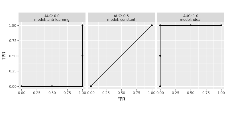
We can see in the figure above three ROC curves, and their corresponding AUC values. Two of the curves have five points, which is the max possible for four samples (no tied scores); the curve for model=constant has two points, which is the min possible (all tied scores).
Derivative of log loss
Many algorithms for learning f are based on gradient descent, which
attempts to minimize a loss function that measures how well f works
for predicting the train data. But gradient descent does not work with
the zero-one loss, because its derivative is zero almost everywhere
(no information to learn how to update parameters to get better
predictions). So instead people use the logistic (cross-entropy)
loss, or the hinge loss, which have linear tails (gradient is -1 when
prediction is bad, which tells the learning algorithm to increase
those predictions). It is computed as in the code below, for each observation:
def log_loss(pred_tensor, label_tensor):
    return torch.log(1+torch.exp(-label_tensor*pred_tensor))
log_loss(four_pred, four_labels)
## tensor([2.1269, 0.0298, 1.3133, 0.2014])
The code below computes the mean log loss (same as torch.nn.BCEWithLogitsLoss) over all samples:
def mean_log_loss(pred_tensor, label_tensor):
    return log_loss(pred_tensor, label_tensor).mean()
mean_log_loss(four_pred, four_labels)
## tensor(0.9178)
mean_log_loss_torch = torch.nn.BCEWithLogitsLoss()
mean_log_loss_torch(four_pred, torch.where(four_labels==1, 1.0, 0.0))
## tensor(0.9178)
And the code below computes the proportion incorrectly classified samples (error rate):
def prop_incorrect(pred_tensor, label_tensor):
    return zero_one_loss(pred_tensor, label_tensor).float().mean()
prop_incorrect(four_pred, four_labels)
## tensor(0.5000)
These functions and their gradients can be visualized using the code below.
log_grad_df_list = []
pred_grid = np.arange(-4.0, 4, 0.5)
for objective in "prop_incorrect", "mean_log_loss":
    ofun = eval(objective)
    for pred_val in pred_grid:
        pred_tensor=torch.tensor([pred_val])
        pred_tensor.requires_grad = True
        label_tensor = torch.tensor([1.0])
        loss = ofun(pred_tensor, label_tensor)
        try:
            loss.backward()
            g_vec = pred_tensor.grad
        except:
            g_val = 0.0 if pred_val != 0 else torch.nan
            g_vec = torch.tensor([g_val])
        log_grad_df_list.append(pd.DataFrame({
            "predicted_score":pred_val,
            "objective":objective,
            "function":["output","derivative"],
            "value":torch.cat([
                loss.reshape(1),
                g_vec.reshape(1)
            ]).detach().numpy(),
        }))
log_grad_df = pd.concat(log_grad_df_list)
gg_log_grad = p9.ggplot()+\
    p9.theme_bw()+\
    p9.geom_hline(
        p9.aes(
            yintercept="value"
        ),
        data=pd.DataFrame({"value":[0]}),
        color="grey"
    )+\
    p9.geom_point(
        p9.aes(
            x="predicted_score",
            y="value",
        ),
        data=log_grad_df
    )+\
    p9.facet_grid("function ~ objective", labeller="label_both")
show("gg_log_grad")
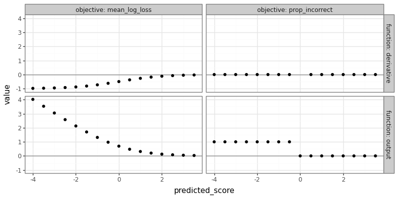
The figure above shows that the log loss (for a positive label) outputs linear tails for negative predicted scores, which means a derivative of -1 that can be used to find model parameters that result in better predictions, in the context of gradient descent learning algorithms. In contrast, the proportion incorrect is a step function, with derivative 0 almost everywhere (except when predicted score is 0, where it is undefined).
Proposed AUM loss for ROC optimization
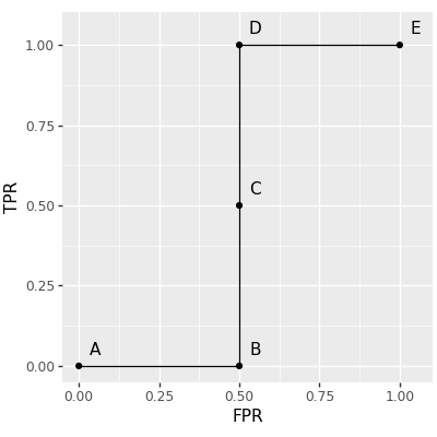
The log loss can be intepreted as a differentiable surrogate for the zero-one loss. There is no derivative for the zero-one loss, so the next best thing is to learn using the log loss, which is a convex/L1 relaxation (L1 meaning the log loss has linear tails and constant gradient). Is it possible to do something similar with the ROC AUC? Yes! Recently in JMLR23 we proposed a new loss function called the AUM, Area Under Min of False Positive and False Negative rates. We showed that is can be interpreted as a L1 relaxation of the sum of min of False Positive and False Negative rates, over all points on the ROC curve. We additionally showed that AUM is piecewise linear, and differentiable almost everywhere, so can be used in gradient descent learning algorithms. Finally, we showed that minimizing AUM encourages points on the ROC curve to move toward the upper left, thereby encouraging large AUC. Computation of the AUM loss requires first computing ROC curves (same as above), which we visualize below using a letter next to each point on the curve:
roc_efficient_df["letter"]=["A","B","C","D","E"]
gg_roc_efficient = gg_roc_inefficient+\
    p9.geom_text(
        p9.aes(
            x="FPR+0.05",
            y="TPR+0.05",
            label="letter",
        ),
        data=roc_efficient_df
    )
show("gg_roc_efficient")
The AUM loss is defined as the area under the minimum of False Positive and False Negative rates, which are the same data we used to compute the ROC curve, and can be visualized using the code below:
roc_long = pd.melt(
    roc_efficient_df,
    value_vars=["FPR","FNR","min(FPR,FNR)"],
    id_vars=["min_constant","max_constant"])
roc_efficient_df["xtext"]=np.where(
    roc_efficient_df["min_constant"] == -np.inf,
    roc_efficient_df["max_constant"]-1,
    np.where(
        roc_efficient_df["max_constant"] == np.inf,
        roc_efficient_df["min_constant"]+1,
        (roc_efficient_df["min_constant"]+roc_efficient_df["max_constant"])/2))
gg_error_funs = p9.ggplot()+\
    p9.theme_bw()+\
    p9.geom_rect(
        p9.aes(
            xmin="min_constant",
            xmax="max_constant",
            ymin="0",
            ymax="min(FPR,FNR)"
        ),
        data=roc_efficient_df)+\
    p9.geom_vline(
        p9.aes(
            xintercept="min_constant",
        ),
        color="grey",
        data=roc_efficient_df)+\
    p9.geom_text(
        p9.aes(
            x="xtext",
            y="0.75",
            label="letter"
        ),
        data=roc_efficient_df)+\
    p9.geom_segment(
        p9.aes(
            x="min_constant",
            xend="max_constant",
            y="value",
            yend="value",
            color="variable",
            size="variable"
        ),
        data=roc_long)+\
    p9.scale_color_manual(
        values={
            "FPR":"red",
            "FNR":"deepskyblue",
            "min(FPR,FNR)":"black"
        })+\
    p9.scale_size_manual(
        values={
            "FPR":3,
            "FNR":5,
            "min(FPR,FNR)":1,
        })+\
    p9.xlab("Constant added to predicted values")+\
    p9.scale_y_continuous(name="value", breaks=[0,0.5,1])
show("gg_error_funs")
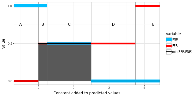
The figure above shows three piecewise constant functions of the constant added to predicted values: FPR, FNR, and their minimum. The AUM is shown in the figure above as the shaded grey region, under the black min function. To compute the AUM, we can use the code below, which first computes the ROC curve.
def Proposed_AUM(pred_tensor, label_tensor):
    """Area Under Min(FP,FN)

    Differentiable loss function for imbalanced binary classification
    problems. Minimizing AUM empirically results in maximizing Area
    Under the ROC Curve (AUC). Arguments: pred_tensor and label_tensor
    should both be 1d tensors, vectors of real-valued predictions and
    integer labels for each observation in the set/batch. Labels
    should be either 1 for positive class or any other value for
    negative class.

    """
    roc = ROC_curve(pred_tensor, label_tensor)
    min_FPR_FNR = roc["min(FPR,FNR)"][1:-1]
    constant_diff = roc["min_constant"][1:].diff()
    return torch.sum(min_FPR_FNR * constant_diff)
The implementation above uses the ROC_curve sub-routine, to
emphasize the similarity with the AUC computation. The Proposed_AUM
function can be used as a drop-in replacement for the logistic loss
(torch.BCEWithLogitsLoss), as can be seen below:
Proposed_AUM(four_pred, four_labels)
## tensor(1.5000)
The AUM loss and its gradient can be visualized using the setup below.
- We assume there are two samples: one positive label, and one negative label.
- We plot the AUM loss and its gradient (with respect to the two
predicted scores) for a grid different values of
f(x1)(predicted score for positive example), while keeping constantf(x0)(predicted score for negative example). - We represent these in the plot below on an X axis called “Difference between predicted scores” because AUM only depends on the difference/rank of predicted scores (not absolute values).
label_vec = [0, 1]
pred_diff_vec = torch.arange(-2, 2, 0.5)
aum_grad_df_list = []
for pred_diff in pred_diff_vec:
    pred_vec = [0, pred_diff]
    for objective in "Proposed_AUM","ROC_AUC":
        pred_tensor = torch.tensor(pred_vec)
        pred_tensor.requires_grad = True
        label_tensor = torch.tensor(label_vec)
        ofun = eval(objective)
        loss = ofun(pred_tensor, label_tensor)
        try:
            loss.backward()
            g_vec = pred_tensor.grad
        except:
            g_val = 0.0 if pred_diff != 0 else torch.nan
            g_vec = torch.tensor([g_val, g_val])
        aum_grad_df_list.append(pd.DataFrame({
            "pred_diff":pred_diff.numpy(),
            "objective":objective,
            "function":["output","deriv0","deriv1"],
            "value":torch.cat([loss.reshape(1),g_vec]).detach().numpy(),
        }))
aum_grad_df = pd.concat(aum_grad_df_list)
gg_aum_grad = p9.ggplot()+\
    p9.theme_bw()+\
    p9.theme(figure_size=(8,5))+\
    p9.geom_hline(
        p9.aes(
            yintercept="value"
        ),
        data=pd.DataFrame({"value":[0]}),
        color="grey"
    )+\
    p9.geom_point(
        p9.aes(
            x="pred_diff",
            y="value",
        ),
        data=aum_grad_df
    )+\
    p9.facet_grid("function ~ objective", labeller="label_both")+\
    p9.scale_x_continuous(
        name="Difference between predicted scores = f(x1)-f(x0)")
show("gg_aum_grad")
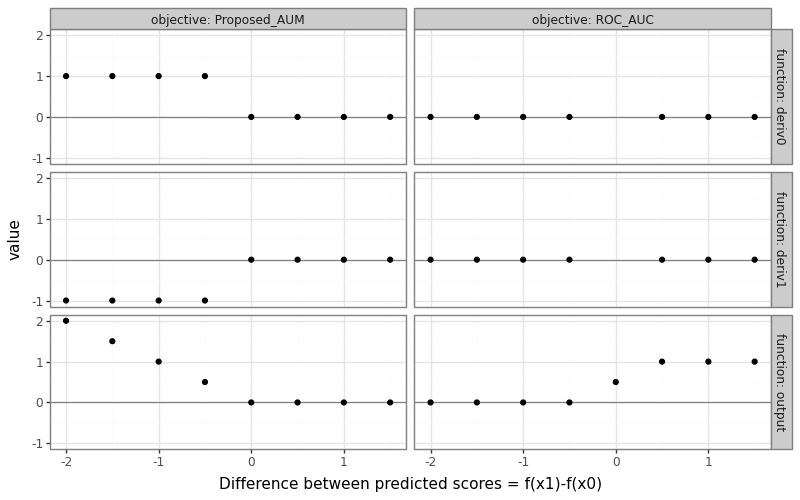
The figure above shows the proposed AUM loss on the left, and the usual ROC AUC objective on the right. We can see that
- The ROC AUC is 0 when the prediction difference is negative, meaning the predicted score for the positive example is less than the predicted score for the negative example (bad/incorrect ranking).
- The ROC AUC derivatives are zero everywhere except when the prediction difference is 0, where they are undefined.
- The AUM increases linearly as the prediction difference gets more negative, so the derivatives are -1 for the positive example, and 1 for the negative example.
- These derivatives mean that the AUM can be decreased by increasing the predicted score for the positive example, or decreasing the predicted score for the negative example.
Conclusions
We have explored the relationship between the zero-one loss and its differentiable surrogate, the logistic loss. We showed how the proposed AUM loss can be interpreted as a differentiable surrogate for the ROC AUC, as shown in the table below.
| Sum over | Piecewise constant | Differentiable Surrogate |
|---|---|---|
| Samples | Zero-one loss | Logistic loss |
| Points on ROC curve | AUC = Area Under ROC Curve | AUM = Area Under Min(FPR,FNR) |
The proposed AUM loss can be implemented in torch code, by first computing the ROC curve, plotting the FPR/FNR as a function of constants added to predicted values, and then summing the Area Under the Min (AUM).
How is AUM different from other differentiable AUC surrogates that sum over all pairs of positive and negative examples? Stay tuned for a new blog post comparing AUM to related work such as Rust and Hocking, Squared Hinge surrogate, LibAUC, etc.
Session info
torch.__version__
## '2.4.1'
np.__version__
## '1.26.0'
p9.__version__
## '0.12.1'