Toby Dylan Hocking | Reshape performance comparison

The goal of this blog post is to explain how to use atime to compare the asymptotic performance (time and memory usage) of different versions of an R package.

Example: wide to long reshape

Data reshaping means changing the shape of the data, in order to get it into a more appropriate format, for learning/plotting/etc. Here we consider wide to long reshape, which means we start with a wide table (many columns) and end up with a long table (fewer columns). One example is the iris data, which starts wide

library(data.table)
(iris.wide <- data.table(iris)[, flower := .I][])

##      Sepal.Length Sepal.Width Petal.Length Petal.Width   Species flower
##             <num>       <num>        <num>       <num>    <fctr>  <int>
##   1:          5.1         3.5          1.4         0.2    setosa      1
##   2:          4.9         3.0          1.4         0.2    setosa      2
##   3:          4.7         3.2          1.3         0.2    setosa      3
##   4:          4.6         3.1          1.5         0.2    setosa      4
##   5:          5.0         3.6          1.4         0.2    setosa      5
##  ---                                                                   
## 146:          6.7         3.0          5.2         2.3 virginica    146
## 147:          6.3         2.5          5.0         1.9 virginica    147
## 148:          6.5         3.0          5.2         2.0 virginica    148
## 149:          6.2         3.4          5.4         2.3 virginica    149
## 150:          5.9         3.0          5.1         1.8 virginica    150

If we wanted to make a histogram of each numeric variable, we first need to reshape, for example using the code below,

(iris.long <- melt(iris.wide, measure.vars = patterns(".*[.].*")))

##        Species flower     variable value
##         <fctr>  <int>       <fctr> <num>
##   1:    setosa      1 Sepal.Length   5.1
##   2:    setosa      2 Sepal.Length   4.9
##   3:    setosa      3 Sepal.Length   4.7
##   4:    setosa      4 Sepal.Length   4.6
##   5:    setosa      5 Sepal.Length   5.0
##  ---                                    
## 596: virginica    146  Petal.Width   2.3
## 597: virginica    147  Petal.Width   1.9
## 598: virginica    148  Petal.Width   2.0
## 599: virginica    149  Petal.Width   2.3
## 600: virginica    150  Petal.Width   1.8

The output above is a table with 600 rows, which is four times the usual 150 rows in the iris data, because we have reshaped the four numeric columns. Using this format, we can create a multi-panel histogram using the code below,

library(ggplot2)
ggplot()+
  geom_histogram(aes(
    value),
    data=iris.long)+
  facet_wrap(~variable)

## `stat_bin()` using `bins = 30`. Pick better value with `binwidth`.

plot of chunk irisHist

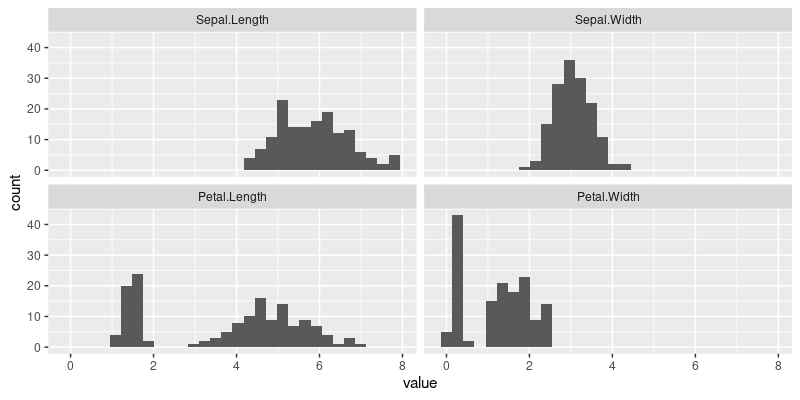
The figure above shows a panel for each numeric variable in the iris data, with a histogram in each panel.

Reshape using nc package

nc, short for named capture, is a package which supports wide to long data reshaping, using the capture_melt_single and capture_melt_multiple functions, such as in the code below,

nc::capture_melt_single(iris.wide, variable=".*[.].*")

##        Species flower     variable value
##         <fctr>  <int>       <char> <num>
##   1:    setosa      1 Sepal.Length   5.1
##   2:    setosa      2 Sepal.Length   4.9
##   3:    setosa      3 Sepal.Length   4.7
##   4:    setosa      4 Sepal.Length   4.6
##   5:    setosa      5 Sepal.Length   5.0
##  ---                                    
## 596: virginica    146  Petal.Width   2.3
## 597: virginica    147  Petal.Width   1.9
## 598: virginica    148  Petal.Width   2.0
## 599: virginica    149  Petal.Width   2.3
## 600: virginica    150  Petal.Width   1.8

The result above is exactly the same as from melt. In fact, nc uses data.table::melt under the hood, so will benefit from the improvements I proposed, which are currently merged into the data.table master branch on GitHub, and which will hopefully soon appear in a CRAN release of data.table (1.15.0).

nc was modified in PR#17 to take advantage of the new features in data.table. The last commit in that PR has SHA1 hash eecced8ea46fbd26c295293fe70e761561a27726. That version of capture_melt_single returns the result of data.table::melt, and the measure.vars argument has meta-data about the variable columns, computed by measure_single.
The first commit in that PR has SHA1 hash 8a045299302bd431eb9dcfacca83c2cd0e83600d, and just modifies a test. That version of the code uses a join to combine variable column meta-data with reshaped data columns, and is less efficient.

In this blog post we will compare the computational efficiency of these two versions of nc. But first, here we explain the advantages of the new reshape features. Consider the code below, which does a similar reshape as above, but with two named arguments (part and dim) instead of one (variable).

nc::capture_melt_single(iris.wide, part=".*", "[.]", dim=".*")

##        Species flower   part    dim value
##         <fctr>  <int> <char> <char> <num>
##   1:    setosa      1  Sepal Length   5.1
##   2:    setosa      2  Sepal Length   4.9
##   3:    setosa      3  Sepal Length   4.7
##   4:    setosa      4  Sepal Length   4.6
##   5:    setosa      5  Sepal Length   5.0
##  ---                                     
## 596: virginica    146  Petal  Width   2.3
## 597: virginica    147  Petal  Width   1.9
## 598: virginica    148  Petal  Width   2.0
## 599: virginica    149  Petal  Width   2.3
## 600: virginica    150  Petal  Width   1.8

The result above has a column for each named argument (part and dim), in which the values come from the text captured by the regular expression, from the corresponding substring of the column name (Sepal/Length/Petal/Width). In the old version of nc, the result above was computed by first doing the reshape, then doing a join with the meta-data from the regular expression parsing of column names (relatively inefficient because of the join/copy). In the new version of nc, we use the new data table reshape feature, which allows meta-data columns (part and dim) to be created at the same time as the reshape table (no copy necessary). The analogous new data.table::melt code would be:

melt(iris.wide, measure.vars=measure(part, dim, pattern="(.*)[.](.*)"))

##        Species flower   part    dim value
##         <fctr>  <int> <char> <char> <num>
##   1:    setosa      1  Sepal Length   5.1
##   2:    setosa      2  Sepal Length   4.9
##   3:    setosa      3  Sepal Length   4.7
##   4:    setosa      4  Sepal Length   4.6
##   5:    setosa      5  Sepal Length   5.0
##  ---                                     
## 596: virginica    146  Petal  Width   2.3
## 597: virginica    147  Petal  Width   1.9
## 598: virginica    148  Petal  Width   2.0
## 599: virginica    149  Petal  Width   2.3
## 600: virginica    150  Petal  Width   1.8

Note that the result above is the same, and the pattern is slightly different. In data.table::measure() we need to specify each capture group using a pair of parentheses (typical for regex engines), whereas in nc we simply use named arguments (no parentheses necessary).

Comparison code

In this section we compare the computational efficiency of the different reshape operations explained above. To explore computational efficiency, we will need to compute time/memory usage for different data sizes. To do that with the iris data, we will generate index vectors of a given size, as below.

N <- 200
(row.numbers <- rep(1:nrow(iris), l=N))

##   [1]   1   2   3   4   5   6   7   8   9  10  11  12  13  14  15  16  17  18  19  20  21  22  23  24  25  26  27  28
##  [29]  29  30  31  32  33  34  35  36  37  38  39  40  41  42  43  44  45  46  47  48  49  50  51  52  53  54  55  56
##  [57]  57  58  59  60  61  62  63  64  65  66  67  68  69  70  71  72  73  74  75  76  77  78  79  80  81  82  83  84
##  [85]  85  86  87  88  89  90  91  92  93  94  95  96  97  98  99 100 101 102 103 104 105 106 107 108 109 110 111 112
## [113] 113 114 115 116 117 118 119 120 121 122 123 124 125 126 127 128 129 130 131 132 133 134 135 136 137 138 139 140
## [141] 141 142 143 144 145 146 147 148 149 150   1   2   3   4   5   6   7   8   9  10  11  12  13  14  15  16  17  18
## [169]  19  20  21  22  23  24  25  26  27  28  29  30  31  32  33  34  35  36  37  38  39  40  41  42  43  44  45  46
## [197]  47  48  49  50

(iris.wide.N <- iris.wide[row.numbers])

##      Sepal.Length Sepal.Width Petal.Length Petal.Width Species flower
##             <num>       <num>        <num>       <num>  <fctr>  <int>
##   1:          5.1         3.5          1.4         0.2  setosa      1
##   2:          4.9         3.0          1.4         0.2  setosa      2
##   3:          4.7         3.2          1.3         0.2  setosa      3
##   4:          4.6         3.1          1.5         0.2  setosa      4
##   5:          5.0         3.6          1.4         0.2  setosa      5
##  ---                                                                 
## 196:          4.8         3.0          1.4         0.3  setosa     46
## 197:          5.1         3.8          1.6         0.2  setosa     47
## 198:          4.6         3.2          1.4         0.2  setosa     48
## 199:          5.3         3.7          1.5         0.2  setosa     49
## 200:          5.0         3.3          1.4         0.2  setosa     50

The output above shows the indices used to construct a data table which will be the input of the wide to long reshape operation. The idea is to do the same as above, but for different sizes N, varying from 10 to 100 to 1000, etc. The code below computes an R expression to execute for each version of nc.

the first argument pkg.path is a path to a git repository containing the R package,
the second argument expr is an R expression, which will be run for each different version of the R package.
the third and fourth arguments specify R package versions (names are identifiers that will appear in plots/output, and values are SHA1 hash values identifying commits).

(nc.expr.list <- atime::atime_versions_exprs(
  pkg.path = "~/R/nc", 
  expr = nc::capture_melt_single(iris.wide.N, part=".*", "[.]", dim=".*"),
  "nc(old)"="8a045299302bd431eb9dcfacca83c2cd0e83600d",
  "nc(new)"="eecced8ea46fbd26c295293fe70e761561a27726"))

## $`nc(old)`
## nc.8a045299302bd431eb9dcfacca83c2cd0e83600d::capture_melt_single(iris.wide.N, 
##     part = ".*", "[.]", dim = ".*")
## 
## $`nc(new)`
## nc.eecced8ea46fbd26c295293fe70e761561a27726::capture_melt_single(iris.wide.N, 
##     part = ".*", "[.]", dim = ".*")

The output above shows how atime works, by replacing each package name double colon prefix in expr (nc::), with a new package name that depends on the commit (for example nc.eecced8ea46fbd26c295293fe70e761561a27726::). In fact atime creates and installs a package with a new name, that depends on the commit, for every version specified. Below we measure asymptotic time/memory usage for the two versions,

The first argument N is a sequence of data sizes,
The second argument setup is an R expression that will be evaluated for each value in N, to create data of a given size,
The third argument expr.list is the list of expressions for which time/memory usage will be measured.
Finally, seconds.limit may optionally be specified. If an expression is slower than this limit for any data size, then no larger data sizes will be measured.

(atime.result <- atime::atime(
  N=10^seq(1, 6, by=0.5),
  setup={
    row.numbers <- rep(1:nrow(iris), l=N)
    iris.wide.N <- iris.wide[row.numbers]
  }, 
  expr.list=nc.expr.list,
  seconds.limit=0.1))

## atime list with 19 measurements for
## nc(new)(N=10 to 316227.766016838)
## nc(old)(N=10 to 1e+05)

plot(atime.result)

plot of chunk atimeResult

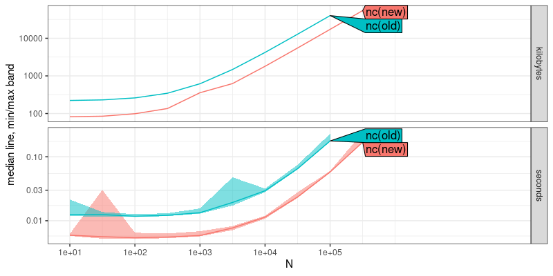
The result above shows that the new version of nc uses less time and memory, by a constant factor (same asymptotic slopes on log-log plot). Below we add asymptotic reference lines, to show the estimated asymptotic time and memory complexity,

(atime.refs <- atime::references_best(atime.result))

## references_best list with 38 measurements, best fit complexity:
## nc(old) (N kilobytes, N seconds)
## nc(new) (N kilobytes, N seconds)

plot(atime.refs)

plot of chunk atimeRefs

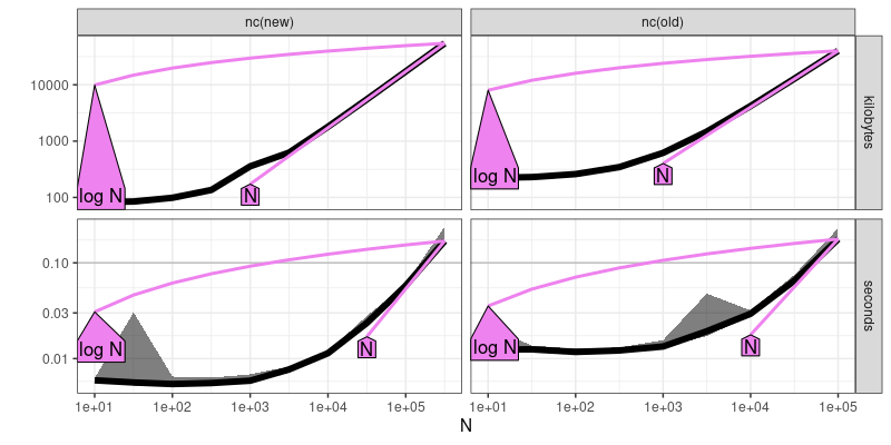
The output and figure above includes violet reference lines, in which the text labels can be interpreted in terms of big O notation (asymptotic time and memory usage). Two violet reference lines are shown (closest upper and lower bound of empirical data). For both new and old versions of nc, linear O(N) seems to be a good fit. A third step/plot is computed below,

(atime.pred <- predict(atime.refs, seconds=0.1, kilobytes=10000))

## atime_prediction object
##         unit expr.name unit.value         N
##       <char>    <char>      <num>     <num>
## 1:   seconds   nc(old)      1e-01  51789.80
## 2:   seconds   nc(new)      1e-01 179941.83
## 3: kilobytes   nc(old)      1e+04  24468.05
## 4: kilobytes   nc(new)      1e+04  57627.11

plot(atime.pred)

## Warning: Transformation introduced infinite values in continuous x-axis

plot of chunk atimePred

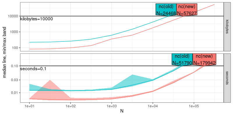
In the plot above, the data size N which can be handled in a given amount of time/memory is shown. It is clear that the new version of nc can handle a larger N for the given time/memory limit.

Comparison with `data.table::melt`

In this section, we explain how to compare nc with the computational requirements for data.table::melt. The simplest method is to simply add another argument to atime, as in the code below.

(atime.melt <- atime::atime(
  N=10^seq(1, 6, by=0.5),
  setup={
    row.numbers <- rep(1:nrow(iris), l=N)
    iris.wide.N <- iris.wide[row.numbers]
  }, 
  expr.list=nc.expr.list,
  melt=melt(iris.wide.N, measure.vars=measure(part, dim, pattern="(.*)[.](.*)")),
  seconds.limit=0.1))

## atime list with 29 measurements for
## melt(N=10 to 316227.766016838)
## nc(new)(N=10 to 316227.766016838)
## nc(old)(N=10 to 1e+05)

plot(atime.melt)

plot of chunk atimeMelt

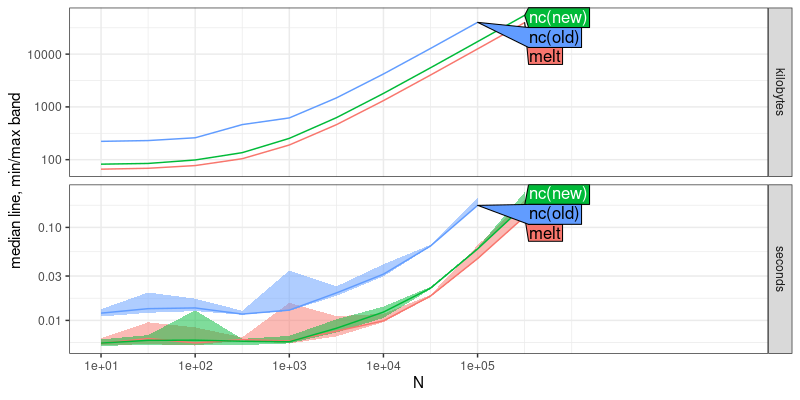
Because the curves in the plot above have the same asymptotic slope, that shows that melt uses the same asymptotic computational resources as nc (but melt is more efficient by a constant factor, which makes sense, because it is used by nc).

Conclusions and Exercises

In this post, we have shown how to use atime to compare asymptotic time and memory usage of R expressions that depend on some data size N. The two kinds of comparisons we explored were different versions of an R package (new and old version of nc), and different packages which implement the same computation (nc versus melt for reshape). Consider doing the exercises below, if you want practice using atime.

In the code above, we used N as the number of rows. Modify the code so that N is used as the number of columns, and make the analogous plots. Are the trends similar?
Another way of comparing melt to nc would be to add the melt code as another expression in the list passed as the expr.list argument to atime. Use quote to add another expression to nc.expr.list, then re-run the comparison above between melt and nc. Is the result the same as when you used the code above? It should be!
If you use melt(measure.vars=measure(part,dim,sep=".")), that is use sep instead of pattern in measure(), is there any difference in computational efficiency?

Session info

sessionInfo()