Ordinary least squares algorithms
The goal of this post is to explore time complexity of various methods for computing least squares regression models.
Introduction
Ordinary least squares regression is a fundamental and classic model in
statistics and in machine learning. When you learn about it in a
stats class, you usually see its computation via the matrix inverse,
but when you look at ?lm in R you see
  method: the method to be used; for fitting, currently only ‘method =
          "qr"’ is supported...
- Arbenz
notes
say that QR time complexity is
O(N^3) - R
?solvesays LAPACK dgesv is used, which says LU decomposition is used, which is same complexity as matrix multiplication, typicallyO(N^3)as well. - Note that these asymptotic time complexity statements are for N =
number of columns of the design matrix X, because solve/LU/QR
operates on X’X, which is a square matrix with dimensions equal to
the number of columns of the design matrix X. That can be confusing,
since in stats/ML we typically use N to denote the number of rows of
X, and P (or D) to denote the number of columns. Both are different
from the N argument to
atime()which we use below for empirical estimation of the asymptotic complexity class. Are you confused yet?
So the asymptotic time complexity is the same. Why is QR preferred? For numerical stability, which means that it is more likely to compute a valid result, for numerically unusual inputs.
R implementations
Nrow <- 5
Ncol <- 2
set.seed(1)
X <- matrix(runif(Nrow*Ncol), Nrow, Ncol)
y <- runif(Nrow)
Xt <- t(X)
qres <- qr(X)
rbind(
  LU=as.numeric(solve(Xt %*% X) %*% (Xt %*% y)),
  QR=solve(qres, y),
  lm=as.numeric(coef(lm(y ~ X + 0))))
##        [,1]        [,2]
## LU 0.768795 -0.03883457
## QR 0.768795 -0.03883457
## lm 0.768795 -0.03883457
Above we see the three methods compute the same result.
Only number of rows increases with N
Converting the examples above to atime code below, (with a constant number of columns=2)
Ncol <- 2
atime.vary.rows <- atime::atime(
  setup={
    set.seed(1)
    X <- matrix(runif(N*Ncol), N, Ncol)
    y <- runif(N)
    Xt <- t(X)
    square.mat <- Xt %*% X
  },
  seconds.limit=0.1,
  mult=Xt %*% X,
  invert=solve(square.mat),
  "mult+invert"={
    as.numeric(solve(Xt %*% X) %*% (Xt %*% y))
  },
  QR={
    qres <- qr(X)
    solve(qres, y)
  },
  lm=as.numeric(coef(lm(y ~ X + 0))))
## Warning: Some expressions had a GC in every iteration; so filtering is disabled.
tit.vary.rows <- ggplot2::ggtitle(paste0(
  "Variable number of rows, N = nrow(X), ncol(X)=",Ncol))
plot(atime.vary.rows)+tit.vary.rows
## Loading required namespace: directlabels
## Warning in ggplot2::scale_y_log10("median line, min/max band"): log-10 transformation introduced infinite values.
## Warning in ggplot2::scale_y_log10("median line, min/max band"): log-10 transformation introduced infinite values.
## log-10 transformation introduced infinite values.
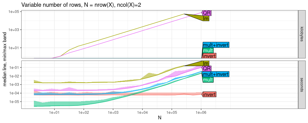
The plot above shows that solve in R (LU decomposition, LAPACK
dgesv) is fastest, looks like by constant factors. The code below
estimates asymptotic time complexity.
refs.vary.rows <- atime::references_best(atime.vary.rows)
plot(refs.vary.rows)+tit.vary.rows
## Warning in ggplot2::scale_y_log10(""): log-10 transformation introduced infinite values.
## Warning in (function (..., deparse.level = 1) : number of rows of result is not a multiple of vector length (arg 2)
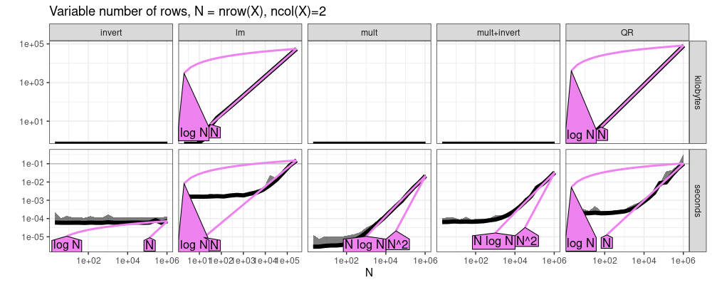
The plot above shows almost linear trends for all methods, except
invert is constant. Is this consistent with the cubic O(N^3)
complexity which we said should be expected? Yes, because the N in
O(N^3) is actually the number of columns of X, which is constant=2
in this example. So it makes sense that the matrix inversion is
asymptotically constant time. The slow/linear step in the fit is
actually the matrix multiplication.
Only number of columns increases, OLS/lm fit
In this section we keep the number of rows of X fixed to 100, and vary the number of columns.
Nrow <- 100
atime.vary.cols <- atime::atime(
  N=unique(as.integer(10^seq(1, log10(Nrow), l=20))),
  setup={
    set.seed(1)
    X <- matrix(runif(Nrow*N), Nrow, N)
    y <- runif(Nrow)
    Xt <- t(X)
    square.mat <- Xt %*% X
  },
  seconds.limit=0.1,
  mult=Xt %*% X,
  invert=solve(square.mat),
  "mult+invert"={
    as.numeric(solve(Xt %*% X) %*% (Xt %*% y))
  },
  QR={
    qres <- qr(X)
    solve(qres, y)
  },
  lm=as.numeric(coef(lm(y ~ X + 0))))
tit.vary.cols <- ggplot2::ggtitle(paste0(
  "Variable number of cols, N = ncol(X), nrow(X)=",Nrow))
plot(atime.vary.cols)+tit.vary.cols
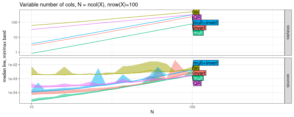
The plot above shows some interesting trends, but I don’t think they
should be interpreted as usual asymptotic timings plots, in which we
may expect that running for a larger N would let us see lm/QR memory
get smaller than LU/invert/mult. Because N is bounded by nrow(X)=r
Nrow, we actually can’t run the code for any N than is already shown
on the plot. The limit is because we can’t invert the X’X matrix if
nrow(X)<ncol(X). In other words, if we run the same code for a
larger Nrow, we get qualitatively the same result (compare memory in
above and below figures).
Nrow <- 300
atime.vary.cols <- atime::atime(
N=unique(as.integer(10^seq(1, log10(Nrow), l=20))),
setup={
set.seed(1)
X <- matrix(runif(Nrow*N), Nrow, N)
y <- runif(Nrow)
Xt <- t(X)
square.mat <- Xt %*% X
},
seconds.limit=0.1,
mult=Xt %*% X,
invert=solve(square.mat),
"mult+invert"={
as.numeric(solve(Xt %*% X) %*% (Xt %*% y))
},
QR={
qres <- qr(X)
solve(qres, y)
},
lm=as.numeric(coef(lm(y ~ X + 0))))
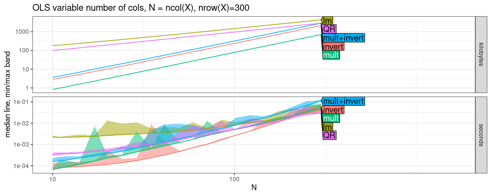
tit.vary.cols <- ggplot2::ggtitle(paste0(
"OLS variable number of cols, N = ncol(X), nrow(X)=",Nrow))
plot(atime.vary.cols)+tit.vary.cols
Only vary number of columns with ridge regression
To get past the limitation of the previous section, we can use a ridge regression fit (L2 regulariztion), so any number of columns can be used with any number of rows.
Nrow <- 100
atime.vary.cols.ridge <- atime::atime(
  setup={
    set.seed(1)
    X <- matrix(runif(Nrow*N), Nrow, N)
    y <- runif(Nrow)
    Xt <- t(X)
    square.mat <- Xt %*% X + diag(N)
  },
  seconds.limit=0.1,
  mult=Xt %*% X,
  invert=solve(square.mat),
  "mult+invert"={
    as.numeric(solve(Xt %*% X+diag(N)) %*% (Xt %*% y))
  },
  QR={
    qres <- qr(X)
    solve(qres, y)
  },
  lm.ridge=as.numeric(coef(MASS::lm.ridge(y ~ X + 0, lambda=1))))
tit.vary.cols.ridge <- ggplot2::ggtitle(paste0(
  "Ridge variable number of cols, N = ncol(X), nrow(X)=",Nrow))
plot(atime.vary.cols.ridge)+tit.vary.cols.ridge
## Warning in ggplot2::scale_y_log10("median line, min/max band"): log-10 transformation introduced infinite values.
## log-10 transformation introduced infinite values.
## log-10 transformation introduced infinite values.
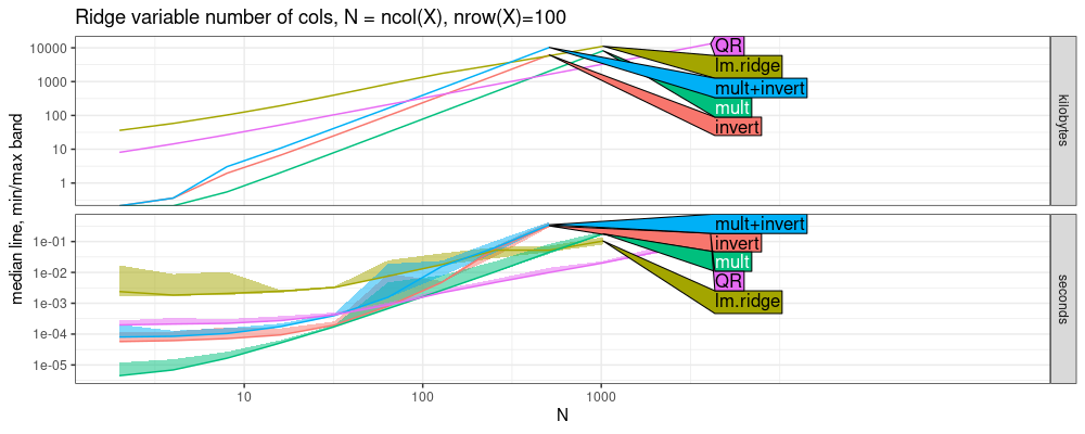
The plot above shows some very interesting trends
QRis fastest, and has smallest slope, same aslm.ridge.- next largest slope is
mult. - largest slopes are
LUandinvert. Below we estimate the asymptotic complexity classes.
refs.vary.cols.ridge <- atime::references_best(atime.vary.cols.ridge)
plot(refs.vary.cols.ridge)+tit.vary.cols.ridge
## Warning in ggplot2::scale_y_log10(""): log-10 transformation introduced infinite values.
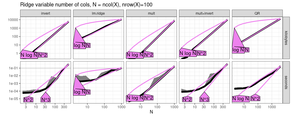
The plot above suggests the following asymptotic complexity classes, as a
function of ncol(X).
lm.ridgeandQRare linear.multis quadratic.invertandLUare cubic.
Both rows and columns increase with N
The code below additionally increases the number of columns.
atime.vary.rows.cols <- atime::atime(
  setup={
    set.seed(1)
    X <- matrix(runif(N*N), N, N)
    y <- runif(N)
    Xt <- t(X)
    square.mat <- Xt %*% X
  },
  seconds.limit=0.1,
  mult=Xt %*% X,
  invert=solve(square.mat),
  "mult+invert"={
    as.numeric(solve(Xt %*% X) %*% (Xt %*% y))
  },
  QR={
    qres <- qr(X)
    solve(qres, y)
  },
  lm=as.numeric(coef(lm(y ~ X + 0))))
tit.vary.rows.cols <- ggplot2::ggtitle(
  "Variable number of rows and cols, N = nrow(X) = ncol(X)")
plot(atime.vary.rows.cols)+tit.vary.rows.cols
## Warning in ggplot2::scale_y_log10("median line, min/max band"): log-10 transformation introduced infinite values.
## log-10 transformation introduced infinite values.
## log-10 transformation introduced infinite values.
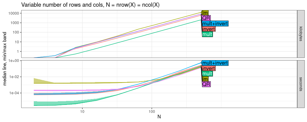
The plot above shows that QR and lm are about the same, which
makes sense, because lm uses QR decomposition method. The difference
between them for small N can be attributed to the overhead of the
lm formula parsing, etc. Both are slightly faster than LU in this case.
Below we estimate asymptotic complexity classes.
refs.vary.rows.cols <- atime::references_best(atime.vary.rows.cols)
plot(refs.vary.rows.cols)+tit.vary.rows.cols
## Warning in ggplot2::scale_y_log10(""): log-10 transformation introduced infinite values.
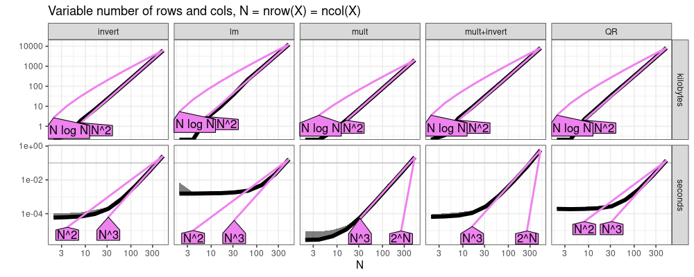
The plot above suggests cubic N^3 asymptotic time for all methods, and
quadratic N^2 asymptotic memory.
Synthesis
Overall our empirical analysis suggests the following time complexity classes
for nrow(X)=N, ncol(X)=P, and M=min(N,P) (rank of X).
| operation | P constant | N constant | vary M=N=P |
|---|---|---|---|
| lm | O(N) | O(P) | O(M^3) |
| QR solve | O(N) | O(P) | O(M^3) |
| mult | O(N) | O(P^2) | O(M^3) |
| invert | O(1) | O(P^3) | O(M^3) |
| mult+invert | O(N) | O(P^3) | O(M^3) |
Is any method clearly faster?
- with lots of data and few features (N>P), all methods are fast/linear (P constant column).
- with lots of features and few data (N<P), lm/QR decomposition is asymptotically faster than matrix multiply and solve/invert/LU (N constant column).
Conclusions
We have shown that there are some asymptotic time/memory differences, between the different methods of estimating ordinary least squares regression coefficients.
Session info
sessionInfo()
## R version 4.4.1 (2024-06-14 ucrt)
## Platform: x86_64-w64-mingw32/x64
## Running under: Windows 11 x64 (build 22631)
##
## Matrix products: default
##
##
## locale:
## [1] LC_COLLATE=English_United States.utf8  LC_CTYPE=English_United States.utf8    LC_MONETARY=English_United States.utf8
## [4] LC_NUMERIC=C                           LC_TIME=English_United States.utf8
##
## time zone: America/Toronto
## tzcode source: internal
##
## attached base packages:
## [1] stats     graphics  utils     datasets  grDevices methods   base
##
## loaded via a namespace (and not attached):
##  [1] directlabels_2024.1.21 vctrs_0.6.5            cli_3.6.3              knitr_1.48             rlang_1.1.4
##  [6] xfun_0.47              highr_0.11             bench_1.1.3            generics_0.1.3         data.table_1.16.99
## [11] glue_1.7.0             nc_2024.9.20           colorspace_2.1-1       scales_1.3.0           fansi_1.0.6
## [16] quadprog_1.5-8         grid_4.4.1             evaluate_0.24.0        munsell_0.5.1          tibble_3.2.1
## [21] MASS_7.3-60.2          profmem_0.6.0          lifecycle_1.0.4        compiler_4.4.1         dplyr_1.1.4
## [26] pkgconfig_2.0.3        atime_2024.8.8         farver_2.1.2           lattice_0.22-6         R6_2.5.1
## [31] tidyselect_1.2.1       utf8_1.2.4             pillar_1.9.0           magrittr_2.0.3         withr_3.0.1
## [36] tools_4.4.1            gtable_0.3.5           ggplot2_3.5.1