Overhead of auto-grad in torch
The goal of this post is to show how to use R torch to compute AUM (Area Under Min of False Positive and False Negative rates, our newly Proposed surrogate loss for ROC curve optimization).
- Paper: Optimizing ROC Curves with a Sort-Based Surrogate Loss for Binary Classification and Changepoint Detection.
- Slides PDF.
This post is similar to what
we did in a previous blog post using
python. This blog
uses R instead of python, in order to compare the auto-grad from torch
with the “explicit gradient” computed the aum R package.
Introduction to binary classification and ROC curves
In supervised binary classification, our goal is to learn a function
f using training inputs/features x, and outputs/labels y, such
that f(x)=y (on new/test data). To illustrate, the code below
defines a data set with four samples:
four_labels_vec <- c(-1,-1,1,1)
four_pred_vec <- c(2.0, -3.5, -1.0, 1.5)
The first to samples are negative, and the second two are positive. The predicted scores are real numbers, which we threshold at zero to determine a predicted class. The ROC curve shows how the prediction error rates change, as we add constants from negative to positive infinity to the predicted scores. To compute the ROC curve using torch, we can use the code below.
ROC_curve <- function(pred_tensor, label_tensor){
  is_positive = label_tensor == 1
  is_negative = label_tensor != 1
  fn_diff = torch::torch_where(is_positive, -1, 0)
  fp_diff = torch::torch_where(is_positive, 0, 1)
  thresh_tensor = -pred_tensor$flatten()
  sorted_indices = torch::torch_argsort(thresh_tensor)
  fp_denom = torch::torch_sum(is_negative) #or 1 for AUM based on count instead of rate
  fn_denom = torch::torch_sum(is_positive) #or 1 for AUM based on count instead of rate
  sorted_fp_cum = fp_diff[sorted_indices]$cumsum(dim=1)/fp_denom
  sorted_fn_cum = -fn_diff[sorted_indices]$flip(1)$cumsum(dim=1)$flip(1)/fn_denom
  sorted_thresh = thresh_tensor[sorted_indices]
  sorted_is_diff = sorted_thresh$diff() != 0
  sorted_fp_end = torch::torch_cat(c(sorted_is_diff, torch::torch_tensor(TRUE)))
  sorted_fn_end = torch::torch_cat(c(torch::torch_tensor(TRUE), sorted_is_diff))
  uniq_thresh = sorted_thresh[sorted_fp_end]
  uniq_fp_after = sorted_fp_cum[sorted_fp_end]
  uniq_fn_before = sorted_fn_cum[sorted_fn_end]
  FPR = torch::torch_cat(c(torch::torch_tensor(0.0), uniq_fp_after))
  FNR = torch::torch_cat(c(uniq_fn_before, torch::torch_tensor(0.0)))
  list(
    FPR=FPR,
    FNR=FNR,
    TPR=1 - FNR,
    "min(FPR,FNR)"=torch::torch_minimum(FPR, FNR),
    min_constant=torch::torch_cat(c(torch::torch_tensor(-Inf), uniq_thresh)),
    max_constant=torch::torch_cat(c(uniq_thresh, torch::torch_tensor(Inf))))
}
four_labels <- torch::torch_tensor(four_labels_vec)
four_pred <- torch::torch_tensor(four_pred_vec)
list.of.tensors <- ROC_curve(four_pred, four_labels)
data.frame(lapply(list.of.tensors, torch::as_array))
##   FPR FNR TPR min.FPR.FNR. min_constant max_constant
## 1 0.0 1.0 0.0          0.0         -Inf         -2.0
## 2 0.5 1.0 0.0          0.5         -2.0         -1.5
## 3 0.5 0.5 0.5          0.5         -1.5          1.0
## 4 0.5 0.0 1.0          0.0          1.0          3.5
## 5 1.0 0.0 1.0          0.0          3.5          Inf
The table above also has one row for each point on the ROC curve, and the following columns:
FPRis the False Positive Rate (X axis of ROC curve plot),TPRis the True Positive Rate (Y axis of ROC curve plot),FNR=1-TPRis the False Negative Rate,min(FPR,FNR)is the minimum ofFPRandFNR,- and
min_constant,max_constantgive the range of constants which result in the corresponding error values. For example, the second row means that adding any constant between -2 and -1.5 results in predicted classes that give FPR=0.5 and TPR=0.
How do we interpret the ROC curve? An ideal ROC curve would
- start at the bottom left (FPR=TPR=0, every sample predicted negative),
- and then go straight to the upper left (FPR=0,TPR=1, every sample predicted correctly),
- and then go straight to the upper right (FPR=TPR=1, every sample predicted positive),
- so it would have an Area Under the Curve of 1.
So when we do ROC analysis, we can look at the curves, to see how close they get to the upper left, or we can just compute the Area Under the Curve (larger is better). To compute the Area Under the Curve, we use the trapezoidal area formula, which amounts to summing the rectangle and triangle under each segment of the curve, as in the code below.
ROC_AUC <- function(pred_tensor, label_tensor){
  roc = ROC_curve(pred_tensor, label_tensor)
  FPR_diff = roc$FPR[2:N]-roc$FPR[1:-2]
  TPR_sum = roc$TPR[2:N]+roc$TPR[1:-2]
  torch::torch_sum(FPR_diff*TPR_sum/2.0)
}
ROC_AUC(four_pred, four_labels)
## torch_tensor
## 0.5
## [ CPUFloatType{} ]
The ROC AUC value is 0.5, indicating that four_pred is not a very
good vector of predictions with respect to four_labels.
Proposed AUM loss for ROC optimization
Recently in JMLR23 we proposed a new loss function called the AUM, Area Under Min of False Positive and False Negative rates. We showed that is can be interpreted as a L1 relaxation of the sum of min of False Positive and False Negative rates, over all points on the ROC curve. We additionally showed that AUM is piecewise linear, and differentiable almost everywhere, so can be used in gradient descent learning algorithms. Finally, we showed that minimizing AUM encourages points on the ROC curve to move toward the upper left, thereby encouraging large AUC. Computation of the AUM loss requires first computing ROC curves (same as above), as in the code below.
Proposed_AUM <- function(pred_tensor, label_tensor){
  roc = ROC_curve(pred_tensor, label_tensor)
  min_FPR_FNR = roc[["min(FPR,FNR)"]][2:-2]
  constant_diff = roc$min_constant[2:N]$diff()
  torch::torch_sum(min_FPR_FNR * constant_diff)
}
The implementation above uses the ROC_curve sub-routine, to
emphasize the similarity with the AUC computation. The Proposed_AUM
function is a differentiable surrogate loss that can be used to
compute gradients. To do that, we first tell torch that the vector of
predicted values requires a gradient, then we call backward() on the
result from Proposed_AUM, which assigns the grad attribute of the
predictions, as can be seen below:
four_pred$requires_grad <- TRUE
(four_aum <- Proposed_AUM(four_pred, four_labels))
## torch_tensor
## 1.5
## [ CPUFloatType{} ][ grad_fn = <SumBackward0> ]
four_pred$grad
## torch_tensor
## [ Tensor (undefined) ]
four_aum$backward()
four_pred$grad
## torch_tensor
##  0.5000
## -0.0000
## -0.5000
## -0.0000
## [ CPUFloatType{4} ]
We can compare the result from auto-grad above, to the result from the
R aum package, which implements a function that gives “explicit
gradients,” actually a dedicated aum_sort C++
function
that computes a matrix of directional derivatives (since AUM has
non-differentiable points). We see that the gradient vector above
(from torch auto-grad) is consistent with the directional derivative
matrix below (from R package aum):
four_labels_diff_dt <- aum::aum_diffs_binary(four_labels_vec, denominator = "rate")
aum::aum(four_labels_diff_dt, four_pred_vec)
## $aum
## [1] 1.5
##
## $derivative_mat
##      [,1] [,2]
## [1,]  0.5  0.5
## [2,]  0.0  0.0
## [3,] -0.5 -0.5
## [4,]  0.0  0.0
##
## $total_error
##   thresh fp_before fn_before
## 1   -2.0       0.0       1.0
## 2    3.5       0.5       0.0
## 3    1.0       0.5       0.5
## 4   -1.5       0.5       1.0
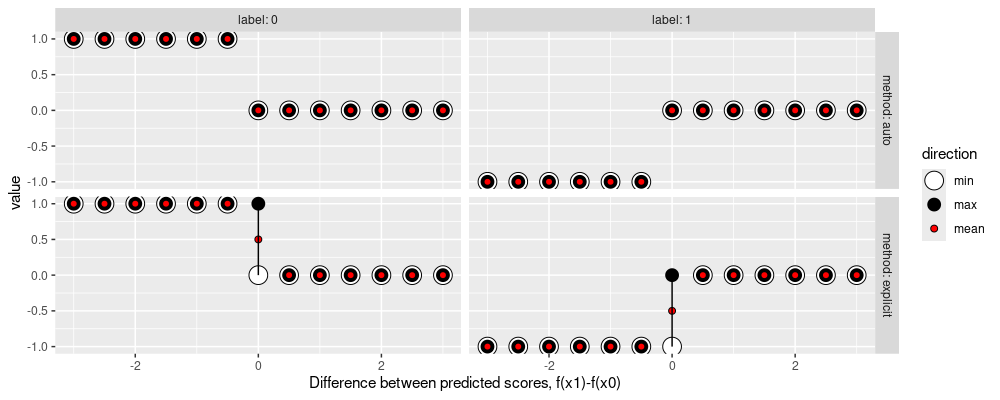
The AUM loss and its gradient can be visualized using the setup below.
- We assume there are two samples: one positive label, and one negative label.
- We plot the AUM loss and its gradient (with respect to the two
predicted scores) for a grid different values of
f(x1)(predicted score for positive example), while keeping constantf(x0)(predicted score for negative example). - We represent these in the plot below on an X axis called “Difference between predicted scores” because AUM only depends on the difference/rank of predicted scores (not absolute values).
label_vec = c(0, 1)
pred_diff_vec = seq(-3, 3, by=0.5)
aum_grad_dt_list = list()
library(data.table)
## data.table 1.16.2 using 1 threads (see ?getDTthreads). Latest news: r-datatable.com
for(pred_diff in pred_diff_vec){
  pred_vec = c(0, pred_diff)
  pred_tensor = torch::torch_tensor(pred_vec)
  pred_tensor$requires_grad = TRUE
  label_tensor = torch::torch_tensor(label_vec)
  loss = Proposed_AUM(pred_tensor, label_tensor)
  loss$backward()
  g_vec = torch::as_array(pred_tensor$grad)
  diff_dt <- aum::aum_diffs_binary(label_vec, denominator = "rate")
  aum_info <- aum::aum(diff_dt, pred_vec)
  grad_list <- list(
    explicit=aum_info$derivative_mat,
    auto=cbind(g_vec, g_vec))
  for(method in names(grad_list)){
    grad_mat <- grad_list[[method]]
    colnames(grad_mat) <- c("min","max")
    aum_grad_dt_list[[paste(pred_diff, method)]] <- data.table(
      label=label_vec, pred_diff, method, grad_mat)
  }
}
(aum_grad_dt <- rbindlist(aum_grad_dt_list)[
, mean := (min+max)/2
][])
##     label pred_diff   method   min   max  mean
##     <num>     <num>   <char> <num> <num> <num>
##  1:     0      -3.0 explicit     1     1   1.0
##  2:     1      -3.0 explicit    -1    -1  -1.0
##  3:     0      -3.0     auto     1     1   1.0
##  4:     1      -3.0     auto    -1    -1  -1.0
##  5:     0      -2.5 explicit     1     1   1.0
##  6:     1      -2.5 explicit    -1    -1  -1.0
##  7:     0      -2.5     auto     1     1   1.0
##  8:     1      -2.5     auto    -1    -1  -1.0
##  9:     0      -2.0 explicit     1     1   1.0
## 10:     1      -2.0 explicit    -1    -1  -1.0
## 11:     0      -2.0     auto     1     1   1.0
## 12:     1      -2.0     auto    -1    -1  -1.0
## 13:     0      -1.5 explicit     1     1   1.0
## 14:     1      -1.5 explicit    -1    -1  -1.0
## 15:     0      -1.5     auto     1     1   1.0
## 16:     1      -1.5     auto    -1    -1  -1.0
## 17:     0      -1.0 explicit     1     1   1.0
## 18:     1      -1.0 explicit    -1    -1  -1.0
## 19:     0      -1.0     auto     1     1   1.0
## 20:     1      -1.0     auto    -1    -1  -1.0
## 21:     0      -0.5 explicit     1     1   1.0
## 22:     1      -0.5 explicit    -1    -1  -1.0
## 23:     0      -0.5     auto     1     1   1.0
## 24:     1      -0.5     auto    -1    -1  -1.0
## 25:     0       0.0 explicit     0     1   0.5
## 26:     1       0.0 explicit    -1     0  -0.5
## 27:     0       0.0     auto     0     0   0.0
## 28:     1       0.0     auto     0     0   0.0
## 29:     0       0.5 explicit     0     0   0.0
## 30:     1       0.5 explicit     0     0   0.0
## 31:     0       0.5     auto     0     0   0.0
## 32:     1       0.5     auto     0     0   0.0
## 33:     0       1.0 explicit     0     0   0.0
## 34:     1       1.0 explicit     0     0   0.0
## 35:     0       1.0     auto     0     0   0.0
## 36:     1       1.0     auto     0     0   0.0
## 37:     0       1.5 explicit     0     0   0.0
## 38:     1       1.5 explicit     0     0   0.0
## 39:     0       1.5     auto     0     0   0.0
## 40:     1       1.5     auto     0     0   0.0
## 41:     0       2.0 explicit     0     0   0.0
## 42:     1       2.0 explicit     0     0   0.0
## 43:     0       2.0     auto     0     0   0.0
## 44:     1       2.0     auto     0     0   0.0
## 45:     0       2.5 explicit     0     0   0.0
## 46:     1       2.5 explicit     0     0   0.0
## 47:     0       2.5     auto     0     0   0.0
## 48:     1       2.5     auto     0     0   0.0
## 49:     0       3.0 explicit     0     0   0.0
## 50:     1       3.0 explicit     0     0   0.0
## 51:     0       3.0     auto     0     0   0.0
## 52:     1       3.0     auto     0     0   0.0
##     label pred_diff   method   min   max  mean
aum_grad_points <- melt(
  aum_grad_dt,
  measure.vars=c("min","max","mean"),
  variable.name="direction")
library(ggplot2)
ggplot()+
  scale_fill_manual(
    values=c(
      min="white",
      mean="red",
      max="black"))+
  scale_size_manual(
    values=c(
      min=6,
      mean=2,
      max=4))+
  geom_point(aes(
    pred_diff, value, fill=direction, size=direction),
    shape=21,
    data=aum_grad_points)+
  geom_segment(aes(
    pred_diff, min,
    xend=pred_diff, yend=max),
    data=aum_grad_dt)+
  scale_x_continuous(
    "Difference between predicted scores, f(x1)-f(x0)")+
  facet_grid(method ~ label, labeller=label_both)

The figure above shows the sub-differential as a function of difference between predicted scores.
- Label: 0 (left) shows the range of sub-gradients with respect to the predicted score for the negative example,
- Label: 1 (right) shows the range of sub-gradients with respect to the predicted score for the positive example,
- For method: auto (top), the torch auto-grad returns a sub-gradient (min=max).
- For method: explicit, the
derivative_matreturned fromaum::aumis shown. When the difference between predicted scores is 0, there is a non-differentiable point, which can be seen as a range of sub-gradients, frommintomax. For gradient descent, we can usemeanas the “gradient.” - These sub-gradients mean that when the difference between predicted scores is negative, the AUM can be decreased by increasing the predicted score for the positive example, or by decreasing the predicted score for the negative example.
Time comparison
In this section, we compare the computation time of the two methods for computing gradients.
a_res <- atime::atime(
  N=as.integer(10^seq(2,6,by=0.2)),
  setup={
    set.seed(1)
    pred_vec = rnorm(N)
    label_vec = rep(0:1, l=N)
  },
  auto={
    pred_tensor = torch::torch_tensor(pred_vec, "double")
    pred_tensor$requires_grad = TRUE
    label_tensor = torch::torch_tensor(label_vec)
    loss = Proposed_AUM(pred_tensor, label_tensor)
    loss$backward()
    torch::as_array(pred_tensor$grad)
  },
  explicit={
    diff_dt <- aum::aum_diffs_binary(label_vec, denominator = "rate")
    aum.info <- aum::aum(diff_dt, pred_vec)
    rowMeans(aum.info$derivative_mat)
  },
  result = TRUE,
  seconds.limit=1
)
## Warning: Some expressions had a GC in every iteration; so filtering is disabled.
## Warning: Some expressions had a GC in every iteration; so filtering is disabled.
## Warning: Some expressions had a GC in every iteration; so filtering is disabled.
## Warning: Some expressions had a GC in every iteration; so filtering is disabled.
## Warning: Some expressions had a GC in every iteration; so filtering is disabled.
plot(a_res)
## Le chargement a nécessité le package : directlabels

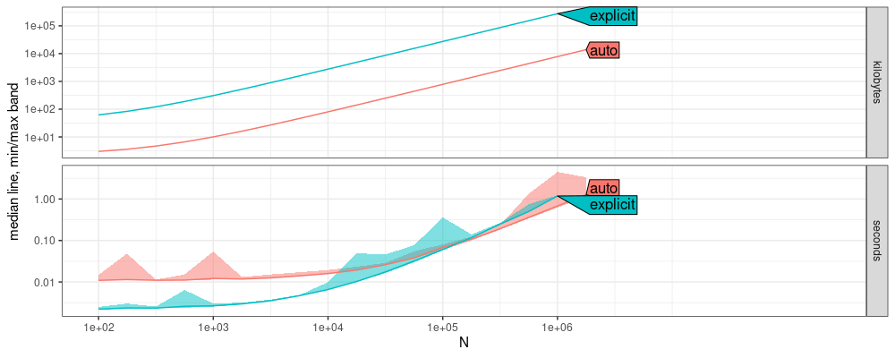
Above we see that auto has about 10x more computation time overhead
than explicit (for small N, less than 1e3). But we see that for
large N (at least 1e5), they have asymptotically the same computation
time. This result implies that auto-grad in torch is actually just as
fast as the explicit gradient computation using the C++ code from R
package aum. We can also see constant factor differences in memory
usage, because atime only measures R memory (not torch memory, so
that usage is under-estimated).
Note that we used torch::torch_tensor(pred_vec, "double") above, for
consistency with R double precision numeric vectors (torch default is
single precision, which can lead to numerical differences for large N,
exercise for the reader, use the code below to explore those
differences).
Below we verify that the results are the same.
res.long <- a_res$measurements[, {
  grad <- result[[1]]
  data.table(grad, i=seq_along(grad))
}, by=.(N,expr.name)]
(res.wide <- dcast(
  res.long, N + i ~ expr.name, value.var="grad"
)[
, diff := auto-explicit
][])
## Key: <N, i>
##                N       i          auto explicit         diff
##            <int>   <int>         <num>    <num>        <num>
##       1:     100       1  0.000000e+00    0e+00 0.000000e+00
##       2:     100       2  0.000000e+00    0e+00 0.000000e+00
##       3:     100       3  0.000000e+00    0e+00 0.000000e+00
##       4:     100       4  0.000000e+00    0e+00 0.000000e+00
##       5:     100       5  2.000004e-02    2e-02 4.053116e-08
##      ---
## 2709530: 1000000  999996  0.000000e+00    0e+00 0.000000e+00
## 2709531: 1000000  999997  0.000000e+00    0e+00 0.000000e+00
## 2709532: 1000000  999998 -1.996756e-06   -2e-06 3.244400e-09
## 2709533: 1000000  999999  2.000481e-06    2e-06 4.808903e-10
## 2709534: 1000000 1000000  0.000000e+00    0e+00 0.000000e+00
res.wide[is.na(diff)]
## Key: <N, i>
## Empty data.table (0 rows and 5 cols): N,i,auto,explicit,diff
dcast(res.wide, N ~ ., list(mean, median, max), value.var="diff")
## Key: <N>
##           N     diff_mean diff_median     diff_max
##       <int>         <num>       <num>        <num>
##  1:     100  0.000000e+00           0 4.053116e-08
##  2:     158  0.000000e+00           0 1.923947e-08
##  3:     251  1.105800e-19           0 2.932927e-08
##  4:     398  6.973763e-20           0 2.276358e-08
##  5:     630  0.000000e+00           0 1.471194e-08
##  6:    1000  0.000000e+00           0 2.574921e-08
##  7:    1584  0.000000e+00           0 2.107235e-08
##  8:    2511  2.417971e-21           0 2.050096e-08
##  9:    3981 -1.443422e-21           0 4.540736e-08
## 10:    6309 -3.436818e-23           0 2.059894e-08
## 11:   10000  0.000000e+00           0 2.641678e-08
## 12:   15848  0.000000e+00           0 1.585646e-08
## 13:   25118  0.000000e+00           0 2.217080e-08
## 14:   39810  0.000000e+00           0 2.172029e-08
## 15:   63095 -3.575141e-22           0 1.886652e-08
## 16:  100000  0.000000e+00           0 2.716064e-08
## 17:  158489 -2.936919e-22           0 1.709201e-08
## 18:  251188  0.000000e+00           0 2.485860e-08
## 19:  398107  6.905837e-24           0 1.699747e-08
## 20:  630957  1.131770e-23           0 1.906540e-08
## 21: 1000000  0.000000e+00           0 2.655792e-08
##           N     diff_mean diff_median     diff_max
The result above shows that there are very little differences between the gradients in the two methods.
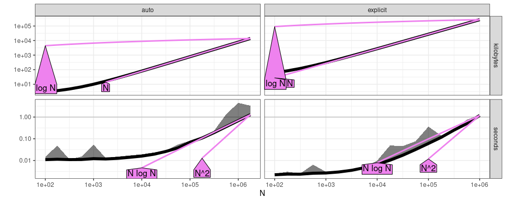
Below we estimate the asymptotic complexity class,
a_refs <- atime::references_best(a_res)
plot(a_refs)

The plot above suggests that memory usage (kilobytes) is linear (N), and computation time (seconds) is linear or log-linear (N log N), which is expected.
Conclusions
We have shown how to compute our proposed AUM using R torch, and
compared the computation time of torch auto-grad with “explicit
gradients” from R package aum. We observed that there is some
overhead to using torch, but asymptotically the two methods take the
same amount of time: log-linear O(N log N), in number of samples N.
Session info
sessionInfo()
## R Under development (unstable) (2024-10-01 r87205)
## Platform: x86_64-pc-linux-gnu
## Running under: Ubuntu 22.04.5 LTS
##
## Matrix products: default
## BLAS:   /usr/lib/x86_64-linux-gnu/blas/libblas.so.3.10.0
## LAPACK: /usr/lib/x86_64-linux-gnu/lapack/liblapack.so.3.10.0
##
## locale:
##  [1] LC_CTYPE=fr_FR.UTF-8       LC_NUMERIC=C               LC_TIME=fr_FR.UTF-8        LC_COLLATE=fr_FR.UTF-8
##  [5] LC_MONETARY=fr_FR.UTF-8    LC_MESSAGES=fr_FR.UTF-8    LC_PAPER=fr_FR.UTF-8       LC_NAME=C
##  [9] LC_ADDRESS=C               LC_TELEPHONE=C             LC_MEASUREMENT=fr_FR.UTF-8 LC_IDENTIFICATION=C
##
## time zone: Europe/Paris
## tzcode source: system (glibc)
##
## attached base packages:
## [1] stats     graphics  utils     datasets  grDevices methods   base
##
## other attached packages:
## [1] ggplot2_3.5.1     data.table_1.16.2
##
## loaded via a namespace (and not attached):
##  [1] bit_4.0.5              gtable_0.3.4           dplyr_1.1.4            compiler_4.5.0         highr_0.11
##  [6] tidyselect_1.2.1       Rcpp_1.0.12            callr_3.7.3            directlabels_2024.1.21 scales_1.3.0
## [11] lattice_0.22-6         R6_2.5.1               labeling_0.4.3         generics_0.1.3         knitr_1.47
## [16] tibble_3.2.1           munsell_0.5.0          atime_2024.12.3        pillar_1.9.0           rlang_1.1.3
## [21] utf8_1.2.4             xfun_0.45              quadprog_1.5-8         bit64_4.0.5            aum_2024.6.19
## [26] cli_3.6.2              withr_3.0.0            magrittr_2.0.3         ps_1.7.6               grid_4.5.0
## [31] processx_3.8.3         torch_0.13.0           lifecycle_1.0.4        coro_1.1.0             vctrs_0.6.5
## [36] bench_1.1.3            evaluate_0.23          glue_1.7.0             farver_2.1.1           profmem_0.6.0
## [41] fansi_1.0.6            colorspace_2.1-0       tools_4.5.0            pkgconfig_2.0.3