Benchmarking a change in data.table
data.table is an R package for efficient data manipulation.
I have an NSF POSE grant about expanding the open-source ecosystem of users and contributors around data.table.
Part of that project is improving performance testing.
The goal of this post is to explain how to use
atime to explore the performance
impact of different versions of a data.table group by operation.
Background
data.table provides a simple syntax for a large number of data manipulation operations: DT[i,j,by] where
iis used to subset rows,jcomputes on columns,byspecifies columns to group by.
Often there are a large number of values of the by columns, and/or
the j computations are time-intensive. In this case, we may have to
wait some time before the computation completes. When using R
interactively, we may wonder how long we have to wait. This was
reported by one user, in
issue#3060.
Joshua Wu is an excellent Google Summer of Code contributor, who is working on fixing this in PR#6228, and I am mentoring him.
Performance
We would like to evaluate the performance (time and memory usage) of
data.table before and after the changes proposed by Joshua in that
PR. Ideally, we should see about the same time and memory usage before
and after. How can we verify that?
I have created the atime R package to help answer performance-related questions like this.
showProgress=TRUE versus FALSE
The PR introduces a new showProgress argument, DT[i,j,by,showProgress], which can be either TRUE or FALSE. We would like to compare the performance of these two options.
First we need to install the code from that PR. The list of commits in that PR currently shows that b3d9a8d151982616ef46bb058554d65c1eb4fbc3 is the last commit, we install that using the code below.
pr.sha <- "b3d9a8d151982616ef46bb058554d65c1eb4fbc3"
repo.sha <- paste0("Rdatatable/data.table@", pr.sha)
remotes::install_github(repo.sha)
## Using github PAT from envvar GITHUB_PAT
## Skipping install of 'data.table' from a github remote, the SHA1 (b3d9a8d1) has not changed since last install.
##   Use `force = TRUE` to force installation
To use atime, we need to do a computation as a function of some data
of size N. In this case N could be the number of rows, or the
number of groups. Let us make N the number of groups,
N <- 5
rows.per.group <- 2
N.rows <- N*rows.per.group
library(data.table)
(DT <- data.table(i=1:N.rows, g=rep(1:N,each=rows.per.group)))
##         i     g
##     <int> <int>
##  1:     1     1
##  2:     2     1
##  3:     3     2
##  4:     4     2
##  5:     5     3
##  6:     6     3
##  7:     7     4
##  8:     8     4
##  9:     9     5
## 10:    10     5
DT[, .(m=mean(i)), by=g]
##        g     m
##    <int> <num>
## 1:     1   1.5
## 2:     2   3.5
## 3:     3   5.5
## 4:     4   7.5
## 5:     5   9.5
The code above computed mean by group for a single data size N (number of groups). To convert that to atime we just
- put the data creation code, which makes
DT, in thesetupargument, - put the code that you want to measure in some other named arguments.
a.result <- atime::atime(
  setup = {
    rows.per.group <- 2
    N.rows <- N*rows.per.group
    DT <- data.table(i=1:N.rows, g=rep(1:N,each=rows.per.group))
  },
  default = DT[, .(m=mean(i)), by=g],
  "TRUE"  = DT[, .(m=mean(i)), by=g, showProgress=TRUE],
  "FALSE" = DT[, .(m=mean(i)), by=g, showProgress=FALSE]
)
The code above has three expressions to measure:
defaultleavesshowProgressunspecified, taking the default value,TRUEandFALSEuse those values forshowProgress.
plot(a.result)
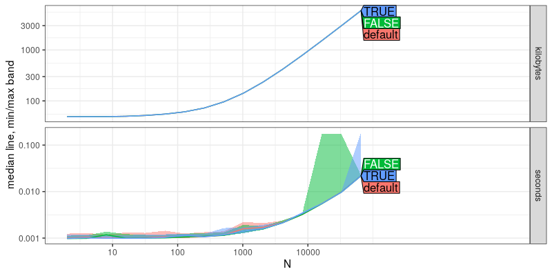
The plot above shows that there is no significant performance difference between the three expressions. This is a good thing!
Comparing versions
We would also like to make sure that the new code is just as fast as the old code (before the PR). So how can we find a version of the code before that PR? First go to the PR commits page, then examine the details of the first commit, 20b213738fdb500369201f6ff584dae3a1bcd44b. That page shows that its parent is 6df30c39cc5d1e910e6f4ab84ccdcc693c64315c, so that is a good candidate.
In summary, we would like to compare the performance of DT[i,j,by] in two different versions of data.table
- 6df30c39cc5d1e910e6f4ab84ccdcc693c64315c is master before adding the showProgress argument,
- b3d9a8d151982616ef46bb058554d65c1eb4fbc3 is the last commit in the PR which adds showProgress.
To compare those two versions of the code, we can use atime_versions
function as below.
edit.data.table <- function(old.Package, new.Package, sha, new.pkg.path) {
  pkg_find_replace <- function(glob, FIND, REPLACE) {
    atime::glob_find_replace(file.path(new.pkg.path, glob), FIND, REPLACE)
  }
  Package_regex <- gsub(".", "_?", old.Package, fixed = TRUE)
  Package_ <- gsub(".", "_", old.Package, fixed = TRUE)
  new.Package_ <- paste0(Package_, "_", sha)
  pkg_find_replace(
    "DESCRIPTION",
    paste0("Package:\\s+", old.Package),
    paste("Package:", new.Package))
  pkg_find_replace(
    file.path("src", "Makevars.*in"),
    Package_regex,
    new.Package_)
  pkg_find_replace(
    file.path("R", "onLoad.R"),
    Package_regex,
    new.Package_)
  pkg_find_replace(
    file.path("R", "onLoad.R"),
    sprintf('packageVersion\\("%s"\\)', old.Package),
    sprintf('packageVersion\\("%s"\\)', new.Package))
  pkg_find_replace(
    file.path("src", "init.c"),
    paste0("R_init_", Package_regex),
    paste0("R_init_", gsub("[.]", "_", new.Package_)))
  pkg_find_replace(
    "NAMESPACE",
    sprintf('useDynLib\\("?%s"?', Package_regex),
    paste0('useDynLib(', new.Package_))
}
v.result <- atime::atime_versions(
  pkg.path="~/R/data.table",
  pkg.edit.fun=edit.data.table,
  seconds.limit=0.1,
  N=as.integer(10^seq(1,9,by=0.5)),
  setup = {
    rows.per.group <- 2
    N.rows <- N*rows.per.group
    DT <- data.table(i=1:N.rows, g=rep(1:N,each=rows.per.group))
  },
  expr = data.table:::`[.data.table`(DT, , .(m=mean(i)), by=g),
  master="6df30c39cc5d1e910e6f4ab84ccdcc693c64315c",
  showProgress=pr.sha)
The code above contains a few new arguments:
pkg.pathis the file path of a git repository containing an R package, in which we can find themasterandshowProgresscommits,pkg.edit.funis a function (here specific todata.table) which is applied to each git version of the package, in order to make it suitable for installation under the namePKG.SHA,seconds.limitis the max number of seconds any timing can take (past which we stop trying larger N). Default is 0.01, and we increased it to 0.1 in the code above.expris an expression which we time for each git SHA version of the package specified. Here there are two versions,masterandshowProgress. Note that inatime_versionswe must writedata.table:::`[.data.table`(DT, , .(m=mean(i)), by=g)instead ofDT[, .(m=mean(i)), by=g], because timing different versions works by substitutingdata.table::with a version-specific package, such asdata.table.6df30c39cc5d1e910e6f4ab84ccdcc693c64315c::. If we usedDT[, .(m=mean(i)), by=g]then it would be using the code in regulardata.tableevery time, instead of the code in one of the version-specific packages likedata.table.6df30c39cc5d1e910e6f4ab84ccdcc693c64315c.
plot(v.result)
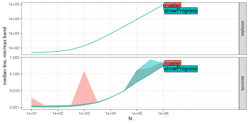
The plot above shows that there is no significant performance
difference between the new showProgress version of the code, and the
previous master version.
Positive control
Above we saw no performance differences between the different versions of the code. Here we study a historical performance improvement.
overall.time <- system.time({
  key.versions <- atime::atime_versions(
    pkg.path="~/R/data.table",
    pkg.edit.fun=edit.data.table,
    N = 10^seq(1, 10, by=0.25),
    setup = {
      set.seed(1)
      L = as.data.table(as.character(rnorm(N, 1, 0.5)))
      setkey(L, V1)
    },
    ## New DT can safely retain key.
    expr = {
      data.table:::`[.data.table`(L, , .SD)
    },
    Fast = "353dc7a6b66563b61e44b2fa0d7b73a0f97ca461", # Close-to-last merge commit in the PR (https://github.com/Rdatatable/data.table/pull/4501/commits) that fixes the issue
    Slow = "3ca83738d70d5597d9e168077f3768e32569c790", # Circa 2024 master parent of close-to-last merge commit (https://github.com/Rdatatable/data.table/commit/353dc7a6b66563b61e44b2fa0d7b73a0f97ca461) in the PR (https://github.com/Rdatatable/data.table/pull/4501/commits) that fixes the issue
    Slower = "cacdc92df71b777369a217b6c902c687cf35a70d") # Circa 2020 parent of the first commit (https://github.com/Rdatatable/data.table/commit/74636333d7da965a11dad04c322c752a409db098) in the PR (https://github.com/Rdatatable/data.table/pull/4501/commits) that fixes the issue
})
plot(key.versions)
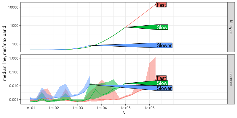
It is clear that there is a significant difference between the three versions (Slower, Slow, Fast).
Note what happens in the code below, when we use expr=L[,.SD]:
atime::atime_versions(
  pkg.path="~/R/data.table",
  pkg.edit.fun=edit.data.table,
  N = 10^seq(1, 10, by=0.5),
  setup = {
    set.seed(1)
    L = as.data.table(as.character(rnorm(N, 1, 0.5)))
    setkey(L, V1)
  },
  expr = L[,.SD],
  Fast = "353dc7a6b66563b61e44b2fa0d7b73a0f97ca461", # Close-to-last merge commit in the PR (https://github.com/Rdatatable/data.table/pull/4501/commits) that fixes the issue
  Slow = "3ca83738d70d5597d9e168077f3768e32569c790", # Circa 2024 master parent of close-to-last merge commit (https://github.com/Rdatatable/data.table/commit/353dc7a6b66563b61e44b2fa0d7b73a0f97ca461) in the PR (https://github.com/Rdatatable/data.table/pull/4501/commits) that fixes the issue
  Slower = "cacdc92df71b777369a217b6c902c687cf35a70d") # Circa 2020 parent of the first commit (https://github.com/Rdatatable/data.table/commit/74636333d7da965a11dad04c322c752a409db098) in the PR (https://github.com/Rdatatable/data.table/pull/4501/commits) that fixes the issue
## Error in (function (pkg.path, expr, sha.vec = NULL, verbose = FALSE, pkg.edit.fun = pkg.edit.default, : expr should contain at least one instance of data.table:: to replace with data.table.353dc7a6b66563b61e44b2fa0d7b73a0f97ca461::
The error message tells us that expr should contain at least one instance of data.table:: to replace with a version-specific package name, data.table.353dc7a6b66563b61e44b2fa0d7b73a0f97ca461::.
Finally, we may wonder from the plot above, just how much faster is the new/Fast version of the code. Looking at the plot above, it is clear that it is quantitatively faster, but it is not clear quantitatively how much faster (10x or 100x?). To answer that question, we can use the predict method as below.
key.refs <- atime::references_best(key.versions)
key.pred <- predict(key.refs)
plot(key.pred)
## Warning in ggplot2::scale_x_log10("N", breaks = meas[, 10^seq(ceiling(min(log10(N))), : log-10 transformation
## introduced infinite values.
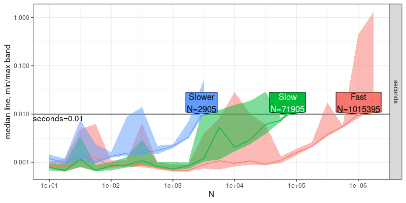
The labels in the plot above show the estimated data size N which are possible to process within the 0.01 second time limit. It shows an estimate of the quantitative differences:
- Slow is about 10x faster than Slower, and
- Fast is about 10x faster than Slow.
Time required
A final advantage to using atime is that it allows us to quickly see asymptotic performance differences between methods which are different by orders of magnitude.
Using the atime approach above, we saw 100x differences (between Slower and Fast methods), but the overall computation time was only a few seconds, as shown below.
overall.time
##    user  system elapsed
##  20.838   0.227  24.435
How does that work? The secret is that atime keeps increasing N until
the time goes over the limit for each method, and then we stop
increasing N for that method. So the computation time for each method
(and the overall time) is never significantly larger than the time
limit. That is true for at least for one trial/timing, but the
default is to run 10 timings (user-controllable via the times
argument). With the default time limit of 0.01, that means atime will
by default take on the order of seconds overall (or less). Most of the time, this default time limit is large enough to see the asymptotic time complexity (not just the constant/overhead time which dominates in the small N regime). For some problems and hardware, this default may need to increase, but so far we have observed that this default is sufficient for seeing significant differences in several different kinds of problems.
In contrast, the traditional method for performance comparison involves comparing the computational requirements for a given data size N (the opposite of the atime approach of comparing the data size N possible for a given time limit). Although that method is simpler to implement (using packages like microbenchmark), it is inherently more time intensive. For example, consider the atime default time limit of 0.01, with a time difference of 100x between methods. Using the traditional approach, assuming the fastest approach takes 0.01 seconds, the slowest approach would take 1 second, and so the overall time is controlled by the slowest approach (whereas the overall time is controlled by the time limit in the atime approach).
And often we have to choose a large N to see the asymptotic regime of the fastest method, so the overall time can be very slow. In the example above, N=1e4 is not large enough to escape the constant/overhead regime, so at least 1e5 is necessary, and maybe 1e6, which takes about 0.01 seconds. For the same data size, Slow takes about 0.1 seconds, and Slower takes about 1 second. And doing that 10 times would mean an overall time of 10-100 seconds, which is an order of magnitude slower than the atime approach (1-10 seconds overall).
Conclusion
We have shown how to use atime to check if there are any performance differences between
- different R code/data, same package version, via
atime(), - different package versions, same R code/data, via
atime_versions().
For future work, you may consider changing setup and the code to
measure, if you think the simple example we considered above is not
actually representative of real use cases.