How reproducible are benchmarks?

data.table is an R package for efficient data manipulation. I have an NSF POSE grant about expanding the open-source ecosystem of users and contributors around data.table. Part of that project is benchmarking time and memory usage, and comparing with similar packages. This post is based on a previous post, and the goal is to see how reproducible those results are, between different computers.

Background about atime

atime is an R package for estimating asymptotic computational requirements, for comparative benchmarking, and for performance testing. In this post we are mostly concerned with comparative benchmarking, which means comparing the time it takes to do a given computation, using different methods. Typical comparative benchmarking uses a single data size N, whereas with atime we use a range of sizes N, until the empirical timing goes over a pre-defined limit. Then we plot the empirical time as a function of N, so we can see asymptotic trends:

• is N large enough to be in the asymptotic regime? (and not the constant overhead regime)
• are the slopes of the asymptotic curves similar or different on the log-log plot? (different slope implies different asymptotic complexity class)
• for which ranges of N would each method be preferable? Or is there a single method which is fastest for all N?

CPUs to compare

On my old MacBook (~2008) running Ubuntu Jammy, cat /proc/cpuinfo says: “Intel(R) Core(TM)2 Duo CPU P7350 @ 2.00GHz.”

My windows computer is from 2018, “Intel(R) Core(TM) i5-9500T CPU @ 2.20GHz.”

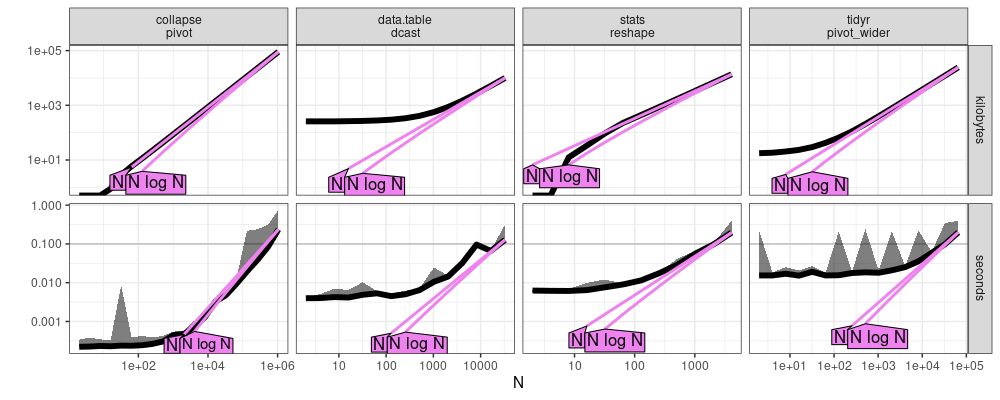
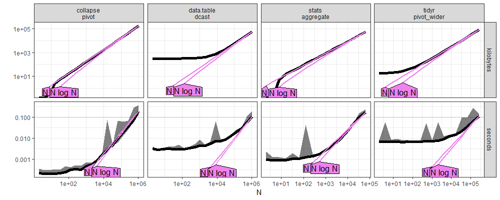
Reshape wide comparison

These comparisons involve tall (sometimes called long) to wide reshape (no aggregation).

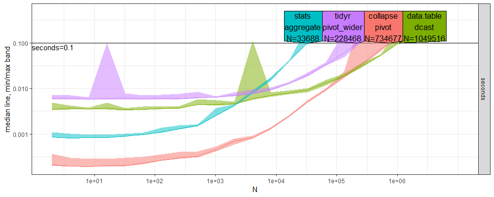
Predict plots

Here we compare the plots which resulted from atime:::plot.atime_prediction.

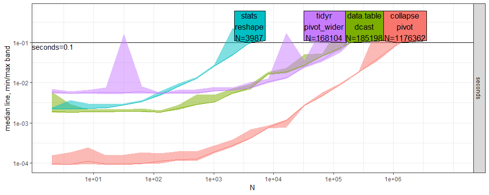
• Above new windows, below old linux.
• We can see, in the direct labels at the top of each plot, that the N values computable within the 0.1 second time limit are quite larger above (about 2-20x).
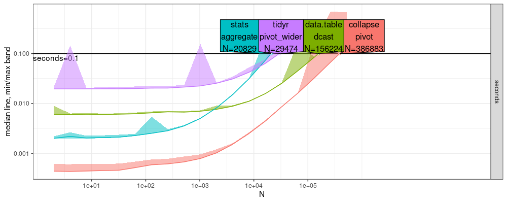
• Overall the qualitative trends are quite similar, in terms of the ordering of the methods. In particular, collapse is fastest, for all N.
• Some trends are not reproducible between CPUs. For example below we see dcast decrease just before the seconds=0.1 limit, whereas we do not see any corresponding decrease above.

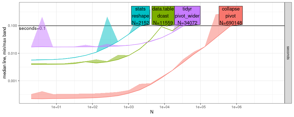
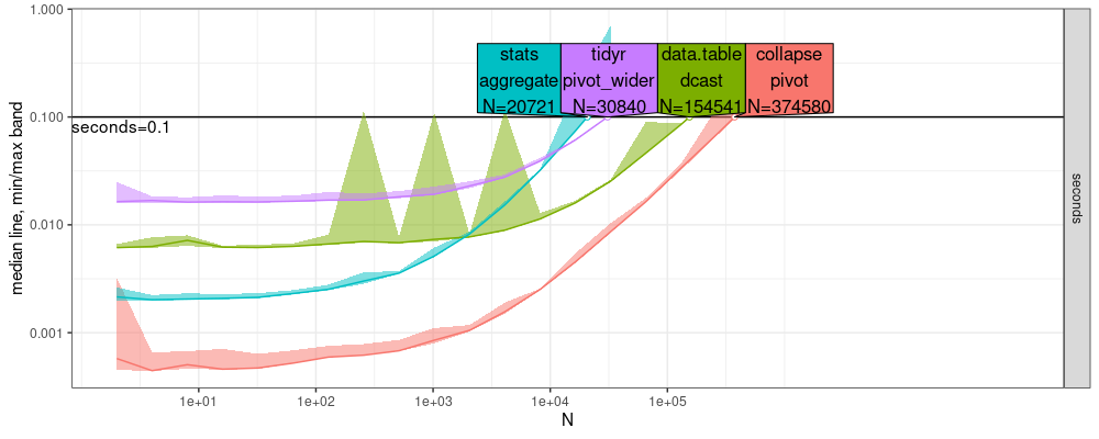
• Above and below are two different runs on the same/old computer.
• we see that the two results are qualitatively very similar (both even have the odd dcast decrease just before the time limit), but differ in the N= values displayed in the direct labels.

References plot

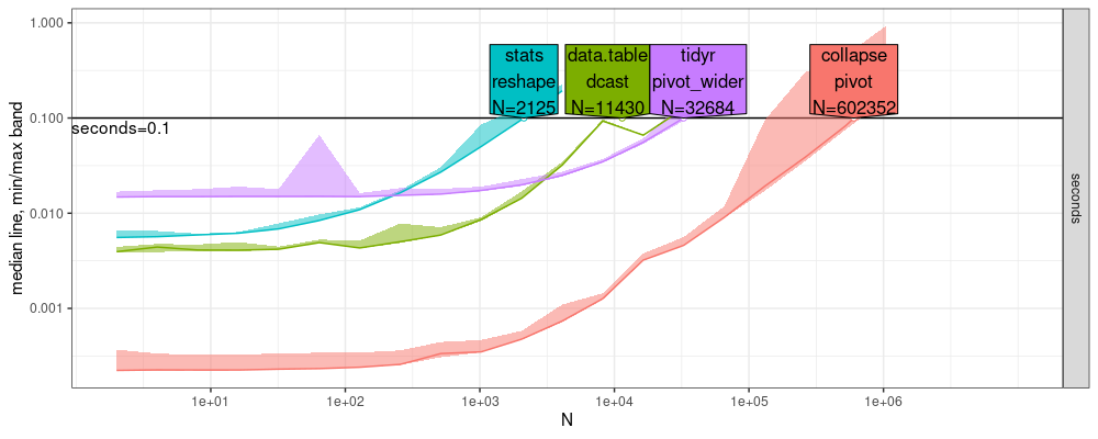
Here we compare the plots which resulted from atime:::plot.references_best.

• Above new windows, below old linux, both look qualitatively similar, but below has the odd dcast decrease just before the time limit.

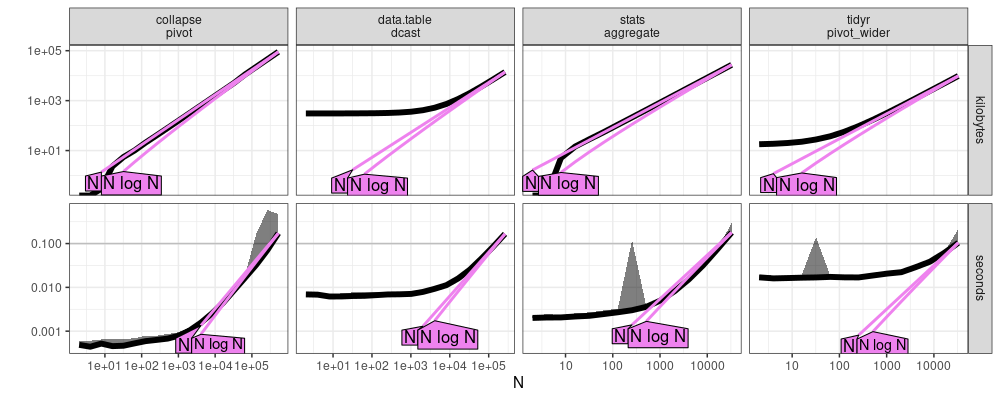
Aggregation comparison

These comparisons involve tall (sometimes called long) to wide reshape, with aggregation by taking the mean of several data.

Predict plots

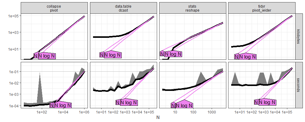
Here we compare the plots which resulted from atime:::plot.atime_prediction.

• Above new windows, below old linux.
• Again the qualitative trends are similar, but there are some subtle differences. For example, in both plots, we see the stats curve crossing both tidyr and data.table curves, but they cross at different N values in the two different plots.
• data.table is fastest for large N above, whereas collapse is fastest for all N below. That is because, in the plot below, we did not increase N large enough to see data.table and collapse cross)

• above and below are two different runs on the same/old computer.
• we see that the two results are qualitatively very similar, but differ in the N= values displayed in the direct labels.

References plot

Here we compare the plots which resulted from atime:::plot.references_best.

• Above new windows, below old linux, a subtle difference is that the curves seem a bit smoother below.

Conclusion

We explored the extent to which atime benchmarks are reproducible between computers. We observed that qualitative trends hold between computers (ordering of methods, which curves cross), but some details may not be reproducible, just like with traditional benchmarks that use a single N value.

cpu details

$ cat /proc/cpuinfo
processor	: 0
vendor_id	: GenuineIntel
cpu family	: 6
model		: 23
model name	: Intel(R) Core(TM)2 Duo CPU     P7350  @ 2.00GHz
stepping	: 6
microcode	: 0x60c
cpu MHz		: 1591.913
cache size	: 3072 KB
physical id	: 0
siblings	: 2
core id		: 0
cpu cores	: 2
apicid		: 0
initial apicid	: 0
fpu		: yes
fpu_exception	: yes
cpuid level	: 10
wp		: yes
flags		: fpu vme de pse tsc msr pae mce cx8 apic sep mtrr pge mca cmov pat pse36 clflush dts acpi mmx fxsr sse sse2 ht tm pbe syscall nx lm constant_tsc arch_perfmon pebs bts rep_good nopl cpuid aperfmperf pni dtes64 monitor ds_cpl vmx est tm2 ssse3 cx16 xtpr pdcm sse4_1 lahf_lm pti tpr_shadow vnmi flexpriority vpid dtherm
vmx flags	: vnmi flexpriority tsc_offset vtpr vapic
bugs		: cpu_meltdown spectre_v1 spectre_v2 spec_store_bypass l1tf mds swapgs itlb_multihit mmio_unknown
bogomips	: 3979.77
clflush size	: 64
cache_alignment	: 64
address sizes	: 36 bits physical, 48 bits virtual
power management: