Implementing optimal partitioning in R
The goal of this post is to show how to implement the optimal partitioning algorithm in R.
Simulate data sequence
The optimal partitioning algorithm (Jackson et al, 2005) is a classic dynamic programming algorithm for change-point detection in sequential data (measured over time or space). To illustrate its computation, we simulate some data below.
set.seed(1)
sim_means <- function(N.segs, N.dim)matrix(
  runif(N.segs*N.dim, 0, 10),
  N.segs, N.dim)
mean.mat <- sim_means(3, 2)
The code above creates a matrix with one column for each dimension of data, and one row for each segment. The code below uses those segment mean values to simulate a certain number of data points per segment, using a normal distribution.
library(data.table)
set.seed(1)
N.per.seg <- 1000
(true.mean.dt <- data.table(
  seg.i=as.integer(row(mean.mat)),
  dim.i=as.integer(col(mean.mat)),
  mean.param=as.numeric(mean.mat)
)[, let(
  first.i=(seg.i-1)*N.per.seg+1,
  last.i=seg.i*N.per.seg,
  parameter="true"
)][, let(
  start=first.i-0.5,
  end=last.i+0.5
)][])
##    seg.i dim.i mean.param first.i last.i parameter  start    end
##    <int> <int>      <num>   <num>  <num>    <char>  <num>  <num>
## 1:     1     1   2.655087       1   1000      true    0.5 1000.5
## 2:     2     1   3.721239    1001   2000      true 1000.5 2000.5
## 3:     3     1   5.728534    2001   3000      true 2000.5 3000.5
## 4:     1     2   9.082078       1   1000      true    0.5 1000.5
## 5:     2     2   2.016819    1001   2000      true 1000.5 2000.5
## 6:     3     2   8.983897    2001   3000      true 2000.5 3000.5
One of the results of the code above is the data table of true means, with one row for each segment and each dimension in the true signal. The other result of the simulation is the table of simulated data, which are shown below,
sim_data <- function(mean.mat, N.per.seg){
  sim.mat <- matrix(NA_real_, nrow(mean.mat)*N.per.seg, ncol(mean.mat))
  for(seg.i in 1:nrow(mean.mat)){
    first.i <- N.per.seg*(seg.i-1)+1
    last.i <- N.per.seg*seg.i
    for(dim.i in 1:ncol(mean.mat)){
      mean.param <- mean.mat[seg.i, dim.i]
      sim.mat[first.i:last.i, dim.i] <- rnorm(N.per.seg, mean.param)
    }
  }
  sim.mat
}
sim.mat <- sim_data(mean.mat, 1000)
data.table(sim.mat)
##             V1        V2
##          <num>     <num>
##    1: 2.028633 10.217043
##    2: 2.838730 10.194010
##    3: 1.819458  8.211300
##    4: 4.250367  9.292809
##    5: 2.984594  9.151474
##   ---
## 2996: 5.891081  7.792324
## 2997: 6.709271  8.652552
## 2998: 5.036394  9.484640
## 2999: 5.725039  8.810420
## 3000: 5.900114  9.241136
To visualize the simulated data, we use the code below.
sim.long <- data.table(
  data.i=as.integer(row(sim.mat)),
  dim.i=as.integer(col(sim.mat)),
  value=as.numeric(sim.mat))
library(ggplot2)
ggplot()+
  facet_grid(dim.i ~ ., labeller=label_both)+
  geom_point(aes(
    data.i, value),
    shape=1,
    data=sim.long)+
  geom_segment(aes(
    start, mean.param,
    color=parameter,
    xend=end, yend=mean.param),
    linewidth=2,
    data=true.mean.dt)+
  scale_x_continuous(
    "Position in data sequence")+
  scale_y_continuous(
    "Data value")
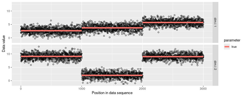
The figure above shows the simulated data (black points) and segment means (orange line segments). The primary goal of change-point detection algorithms like optimal partitioning is to recover the true segment means, using only the noisy simulated data.
Implementing optimal partitioning in R
The goal of the optimal partitioning algorithm is to compute the segmentation with the best cost, given a data set, and a non-negative penalty value. The cost is defined as the total squared error plus a penalty for each change-point added. The main idea of the algorithm is to compute the optimal cost recursively, so we need to initialize a vector of optimal cost values which start as missing, but we will fill in later:
N.data <- nrow(sim.mat)
best.cost.vec <- rep(NA_real_, N.data)
First data point
We start at the first data point, which in this case is:
sim.mat[1,]
## [1] 2.028633 10.217043
In a normal model, the best means are the data themselves, which result in a total squared error of zero, which is our value for the best cost at data point 1:
best.mean1 <- sim.mat[1,]
(best.cost1 <- sum((sim.mat[1,]-best.mean1)^2))
## [1] 0
best.cost.vec[1] <- best.cost1
Second data point, slow computation with mean
The second data point is
sim.mat[2,]
## [1] 2.83873 10.19401
Now, we have a choice. Do we put a change-point between the first and second data points, or not? For the model with no change-point, we compute the cost using the mean matrix below:
(mean.from.1.to.2 <- matrix(
  colMeans(sim.mat[1:2,]),
  nrow=2, ncol=2, byrow=TRUE))
##          [,1]     [,2]
## [1,] 2.433681 10.20553
## [2,] 2.433681 10.20553
The cost is the total squared error:
(cost.from.1.to.2.no.change <- sum((mean.from.1.to.2-sim.mat[1:2,])^2))
## [1] 0.3283939
Second data point, fast computation with cumsum trick
It is difficult to see for the case of only two data points, but the cost computation above is asymptotically slow, because it is linear in the number of data points. We can reduce that to a constant time operation, if we use the cumulative sum trick, with the cost factorization trick. Above we wrote the total squared error as the sum of the squared difference, but using the factorization trick, we can compute it using:
(factorization.mat <- mean.from.1.to.2^2 - 2*mean.from.1.to.2*sim.mat[1:2,] + sim.mat[1:2,]^2)
##           [,1]         [,2]
## [1,] 0.1640643 0.0001326326
## [2,] 0.1640643 0.0001326326
sum(factorization.mat)
## [1] 0.3283939
The calculation above is still O(N), linear time in the number of data, because of the sum over rows. To get that down to constant time, we need to first compute matrices of cumulative sums:
cum.data <- rbind(0,apply(sim.mat,2,cumsum))
cum.squares <- rbind(0,apply(sim.mat^2,2,cumsum))
The code above is O(N) linear time, but it only needs to be computed once in the entire algorithm. Below we use those cumulative sum matrices to compute the cost in constant time.
sum_trick <- function(m, start, end)m[end+1,,drop=FALSE]-m[start,,drop=FALSE]
cost_trick <- function(start, end){
  sum_trick(cum.squares, start, end)-
    sum_trick(cum.data, start, end)^2/
    (end+1-start)
}
(cost.1.2.trick.vec <- cost_trick(1,2))
##           [,1]         [,2]
## [1,] 0.3281287 0.0002652652
sum(cost.1.2.trick.vec)
## [1] 0.3283939
Actually the sum above is O(D), linear in the number of columns/dimensions of data, but constant/independent of N, the number of rows/observations of data (which is the important part for OPART to be fast).
atime comparison
We can verify the constant versus linear time complexity of the two computations using the atime code below:
trick_vs_mean <- atime::atime(
  N=unique(as.integer(10^seq(1, 3, by=0.2))),
  trick=sum(cost_trick(1,N)),
  mean={
    sim.N.mat <- sim.mat[1:N,]
    mean.mat <- matrix(
      colMeans(sim.N.mat),
      nrow=N, ncol=2, byrow=TRUE)
    sum((sim.N.mat-mean.mat)^2)
  },
  result=TRUE)
plot(trick_vs_mean)
## Warning in ggplot2::scale_y_log10("median line, min/max band"): log-10 transformation introduced infinite values.
## log-10 transformation introduced infinite values.
## log-10 transformation introduced infinite values.
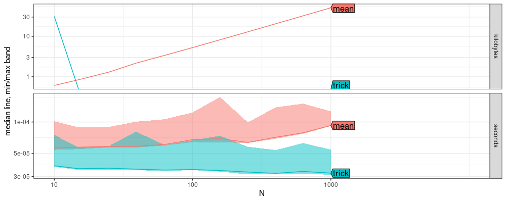
It is clear from the plot above that time and memory usage increase with N for the mean method, but not for the trick method. The code below shows that they get the same result:
(trick_vs_mean_result <- dcast(
  trick_vs_mean$measurements,
  N ~ expr.name,
  value.var="result"))
## Key: <N>
##         N     mean    trick
##     <int>   <list>   <list>
##  1:    10 18.26147 18.26147
##  2:    15   31.101   31.101
##  3:    25  48.7766  48.7766
##  4:    39 68.17109 68.17109
##  5:    63 115.3809 115.3809
##  6:   100 184.8392 184.8392
##  7:   158 280.7583 280.7583
##  8:   251 492.4426 492.4426
##  9:   398 774.3207 774.3207
## 10:   630 1285.341 1285.341
## 11:  1000  2150.46  2150.46
trick_vs_mean_result[, all.equal(mean, trick)]
## [1] TRUE
Second data point, cost of change-point
We also have to consider the model with a change-point. In that case, there are two segments with zero squared error, and so the cost is equal to the penalty. Let’s take a penalty value of
penalty <- 15
So the two options are:
cost.from.1.to.2.no.change
## [1] 0.3283939
(cost.from.1.to.2.change <- penalty)
## [1] 15
We combine them into a vector:
(cost.from.1.to.2.candidates <- c(cost.from.1.to.2.no.change, cost.from.1.to.2.change))
## [1] 0.3283939 15.0000000
We then find the min cost in that vector:
(best.i.from.1.to.2 <- which.min(cost.from.1.to.2.candidates))
## [1] 1
And we end this iteration (for data point 2) by saving these values for the next iteration:
best.change.vec <- rep(NA_integer_, N.data)
best.change.vec[2] <- best.i.from.1.to.2
best.cost.vec[2] <- cost.from.1.to.2.candidates[best.i.from.1.to.2]
data.table(best.cost.vec,best.change.vec)
##       best.cost.vec best.change.vec
##               <num>           <int>
##    1:     0.0000000              NA
##    2:     0.3283939               1
##    3:            NA              NA
##    4:            NA              NA
##    5:            NA              NA
##   ---
## 2996:            NA              NA
## 2997:            NA              NA
## 2998:            NA              NA
## 2999:            NA              NA
## 3000:            NA              NA
Third data point
The third data point is where we can start to see how to write a general and efficient implementation of the optimal partioning algorithm. We want to compute the best model among these candidates:
- last segment starts at data point 1: no changes.
- last segment starts at data point 2: change between data points 1 and 2.
- last segment starts at data point 3: change between data points 2 and 3, and maybe another change before that.
Actually, for the third candidate, we already know that the best model up to data point 2 does not include a change between 1 and 2, and exploiting that existing result is the main idea of the dynamic programming algorithm. To compute the cost of these three candidates, we first compute the cost of the last segment in each candidate:
up.to <- 3
(last.seg.cost <- rowSums(cost_trick(1:up.to, rep(up.to, up.to))))
## [1] 3.231199e+00 2.485026e+00 1.465494e-14
We also need to compute the cost of the other segments, before the last one.
- For the case of the first candidate, there are no other segments, so the cost is zero.
- For the case of the other candidates, we can use the optimal cost which has already been computed (this is dynamic programming), but we need to add the penalty for an additional change-point.
(other.seg.cost <- c(0, best.cost.vec[seq(1, up.to-1)]+penalty))
## [1] 0.00000 15.00000 15.32839
The total cost is the sum of the cost on the last segment, and the other segments:
(total.seg.cost <- last.seg.cost+other.seg.cost)
## [1] 3.231199 17.485026 15.328394
The iteration ends with a minimization:
(best.i.from.1.to.3 <- which.min(total.seg.cost))
## [1] 1
best.change.vec[3] <- best.i.from.1.to.3
best.cost.vec[3] <- total.seg.cost[best.i.from.1.to.3]
data.table(best.cost.vec,best.change.vec)
##       best.cost.vec best.change.vec
##               <num>           <int>
##    1:     0.0000000              NA
##    2:     0.3283939               1
##    3:     3.2311993               1
##    4:            NA              NA
##    5:            NA              NA
##   ---
## 2996:            NA              NA
## 2997:            NA              NA
## 2998:            NA              NA
## 2999:            NA              NA
## 3000:            NA              NA
Other data points
More generally, we can use the for loop below to compute the optimal cost up to any data point,
for(up.to in 1:N.data){
  last.seg.cost <- rowSums(cost_trick(1:up.to, rep(up.to, up.to)))
  change.cost <- if(up.to>1)best.cost.vec[seq(1, up.to-1)]+penalty
  other.seg.cost <- c(0, change.cost)
  total.cost <- other.seg.cost+last.seg.cost
  best.i <- which.min(total.cost)
  best.change.vec[up.to] <- best.i
  best.cost.vec[up.to] <- total.cost[best.i]
}
data.table(change=best.change.vec, cost=best.cost.vec)
##       change         cost
##        <int>        <num>
##    1:      1    0.0000000
##    2:      1    0.3283939
##    3:      1    3.2311993
##    4:      1    6.3419438
##    5:      1    6.4777720
##   ---
## 2996:   2001 6253.5803289
## 2997:   2001 6254.6838822
## 2998:   2001 6255.3987136
## 2999:   2001 6255.4251053
## 3000:   2001 6255.5342708
The table above shows the first/last few rows of the resulting optimal cost and change.
Decoding in R
How can we use the table of optimal cost and change indices to find the optimal segmentation? The last row of the optimal cost/change table tells us where to look for the previous change-point:
(last.seg.start <- best.change.vec[N.data])
## [1] 2001
We see that the last segment starts at the data point given in the result above. We can look at the entry just before that to determine the previous change-point:
(second.to.last.seg.start <- best.change.vec[last.seg.start-1])
## [1] 1001
We see that the second to last segment starts at the data point given in the result above. We can look at the entry just before that to determine the previous change-point:
(third.to.last.seg.start <- best.change.vec[second.to.last.seg.start-1])
## [1] 1
We see the result above is 1, the first data point, so this must be the first segment. This algorithm is commonly known as “decoding” the optimal change position vector, to determine the optimal segmentation. Translating the logic above to a for loop, we get the code below:
seg.dt.list <- list()
last.i <- length(best.change.vec)
while(print(last.i)>0){
  first.i <- best.change.vec[last.i]
  seg.dt.list[[paste(last.i)]] <- data.table(
    first.i, last.i,
    mean=sum_trick(cum.data, first.i, last.i)/(last.i+1-first.i))
  last.i <- first.i-1L
}
## [1] 3000
## [1] 2000
## [1] 1000
## [1] 0
rbindlist(seg.dt.list)[seq(.N,1)]
##    first.i last.i  mean.V1  mean.V2
##      <int>  <int>    <num>    <num>
## 1:       1   1000 2.643438 9.065816
## 2:    1001   2000 3.736548 2.033542
## 3:    2001   3000 5.708470 8.972196
Compare the result above from dynamic programming to the true values from the simulation below:
mean.mat
##          [,1]     [,2]
## [1,] 2.655087 9.082078
## [2,] 3.721239 2.016819
## [3,] 5.728534 8.983897
It is clear that dynamic programming computes a segmentation model with mean values that closely match the true values from the simulation.
Pruning
The Pruned Exact Linear Time (PELT) algorithm of Killick et al. (2012) allows us to prune the set of change-points, while retaining the same optimal solution. To implement that algorithm, we again allocate vectors to store the optimal cost and change-points.
pelt.change.vec <- rep(NA_integer_, N.data)
pelt.cost.vec <- rep(NA_real_, N.data+1)
pelt.cost.vec[1] <- -penalty
Above we initialize the first element of the cost vector to the
negative penalty, so we don’t have to treat the model with no changes
as a special case. We can view pelt.cost.vec[i] as the best cost up
to but not including data point i (and unlike the previous
formulation, we always have to add a penalty to obtain the overall
cost). Below we initialize vectors to store the total number of
candidates considered by the algorithm, as well as the min and max
over all candidates considered:
pelt.candidates.vec <- rep(NA_integer_, N.data)
pelt.candidates.min <- rep(NA_integer_, N.data)
pelt.candidates.max <- rep(NA_integer_, N.data)
We initialize the vector of candidates, then proceed in a loop over data points.
candidate.vec <- 1L
for(up.to in 1:N.data){
  N.cand <- length(candidate.vec)
  pelt.candidates.vec[up.to] <- N.cand
  pelt.candidates.min[up.to] <- min(candidate.vec)
  pelt.candidates.max[up.to] <- max(candidate.vec)
  last.seg.cost <- rowSums(cost_trick(candidate.vec, rep(up.to, N.cand)))
  prev.cost <- pelt.cost.vec[candidate.vec]
  cost.no.penalty <- prev.cost+last.seg.cost
  total.cost <- cost.no.penalty+penalty
  best.i <- which.min(total.cost)
  pelt.change.vec[up.to] <- candidate.vec[best.i]
  total.cost.best <- total.cost[best.i]
  pelt.cost.vec[up.to+1] <- total.cost.best
  candidate.vec <- c(candidate.vec[cost.no.penalty < total.cost.best], up.to+1L)
}
The pruning rule is implemented in the last line of the loop above. We keep only the candidates that have a cost without penalty which is less than the total cost of the best model. We can view the results of the algorithm in the table below:
(pelt.dt <- data.table(
  iteration=seq_along(pelt.change.vec),
  change=pelt.change.vec,
  cost=pelt.cost.vec[-1],
  candidates=pelt.candidates.vec,
  min.candidate=pelt.candidates.min,
  max.candidate=pelt.candidates.max))
##       iteration change         cost candidates min.candidate max.candidate
##           <int>  <int>        <num>      <int>         <int>         <int>
##    1:         1      1    0.0000000          1             1             1
##    2:         2      1    0.3283939          2             1             2
##    3:         3      1    3.2311993          3             1             3
##    4:         4      1    6.3419438          4             1             4
##    5:         5      1    6.4777720          5             1             5
##   ---
## 2996:      2996   2001 6253.5803289        572          2001          2996
## 2997:      2997   2001 6254.6838822        573          2001          2997
## 2998:      2998   2001 6255.3987136        574          2001          2998
## 2999:      2999   2001 6255.4251053        575          2001          2999
## 3000:      3000   2001 6255.5342708        576          2001          3000
Above the “candidate” columns let us analyze the empirical time
complexity of the algorithm (more candidates to consider mean a slower
algorithm). Below we verify that the change and cost columns are
consistent with the values we obtained using OPART.
all.equal(pelt.dt$cost, best.cost.vec)
## [1] TRUE
all.equal(pelt.dt$change, pelt.change.vec)
## [1] TRUE
Below we visualize the change-point candidates that are considered during the two algorithms.
ggplot()+
  geom_point(aes(
    iteration, iteration, color=algorithm),
    size=4,
    data=data.table(pelt.dt, y="number of candidates", algorithm="OPART"))+
  geom_point(aes(
    iteration, candidates, color=algorithm),
    size=2,
    data=data.table(pelt.dt, y="number of candidates", algorithm="PELT"))+
  facet_grid(y ~ ., scales="free")+
  geom_segment(aes(
    iteration, 1,
    color=algorithm,
    xend=iteration, yend=iteration),
    data=data.table(pelt.dt, y="candidate range", algorithm="OPART"))+
  geom_segment(aes(
    iteration, min.candidate,
    color=algorithm,
    xend=iteration, yend=max.candidate),
    data=data.table(pelt.dt, y="candidate range", algorithm="PELT"))
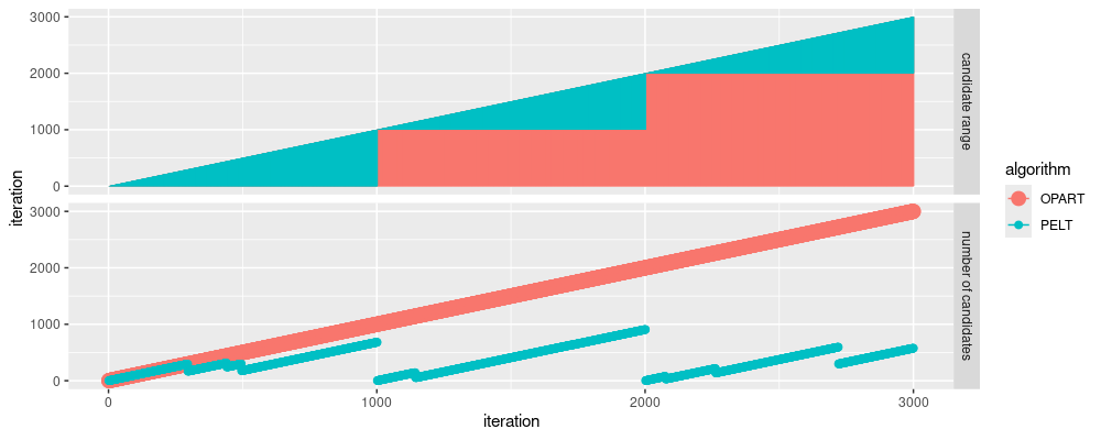
Above we can see two panels:
candidate rangeshows us the min/max of the indices considered for the minimization, in each iteration of the dynamic programming for loop. We see three small triangles along the diagonal for OPART (indicating linear time), and a large triangle for PELT (indicating quadratic time).number of candidatesshows us ho many indices are considered for the minimization, in each iteration of the dynamic programming for loop. We see that the number of candidates never exceeds 1000, because these data have a significant change every 1000 data points. In contrast, the number of candidates considered by OPART grows to the data size (3000).
The figure above clearly shows why the algorithm was named “Linear Time” – the number of candidates considered depends on the number of data points per segment (not the overall number of data points).
Converting to functions
Below we define a function which implements OPART.
OPART <- function(sim.mat, penalty){
  cum.data <- rbind(0, apply(sim.mat, 2, cumsum))
  cum.squares <- rbind(0, apply(sim.mat^2, 2, cumsum))
  sum_trick <- function(m, start, end)m[end+1,,drop=FALSE]-m[start,,drop=FALSE]
  cost_trick <- function(start, end){
    sum_trick(cum.squares, start, end)-
      sum_trick(cum.data, start, end)^2/
      (end+1-start)
  }
  best.change.vec <- rep(NA_integer_, nrow(sim.mat))
  best.cost.vec <- rep(NA_real_, nrow(sim.mat))
  for(up.to in seq(1, nrow(sim.mat))){
    last.seg.cost <- rowSums(cost_trick(1:up.to, rep(up.to, up.to)))
    change.cost <- if(up.to>1)best.cost.vec[seq(1, up.to-1)]+penalty
    other.seg.cost <- c(0, change.cost)
    total.cost <- other.seg.cost+last.seg.cost
    best.i <- which.min(total.cost)
    best.cost <- total.cost[best.i]
    best.change.vec[up.to] <- best.i
    best.cost.vec[up.to] <- best.cost
  }
  list(cost=best.cost.vec, change=best.change.vec, max.candidates=up.to)
}
Below we define a function which implements PELT.
PELT <- function(sim.mat, penalty, prune=TRUE){
  cum.data <- rbind(0, apply(sim.mat, 2, cumsum))
  cum.squares <- rbind(0, apply(sim.mat^2, 2, cumsum))
  sum_trick <- function(m, start, end)m[end+1,,drop=FALSE]-m[start,,drop=FALSE]
  cost_trick <- function(start, end){
    sum_trick(cum.squares, start, end)-
      sum_trick(cum.data, start, end)^2/
      (end+1-start)
  }
  N.data <- nrow(sim.mat)
  pelt.change.vec <- rep(NA_integer_, N.data)
  pelt.cost.vec <- rep(NA_real_, N.data+1)
  pelt.cost.vec[1] <- -penalty
  pelt.candidates.vec <- rep(NA_integer_, N.data)
  candidate.vec <- 1L
  for(up.to in 1:N.data){
    N.cand <- length(candidate.vec)
    pelt.candidates.vec[up.to] <- N.cand
    last.seg.cost <- rowSums(cost_trick(candidate.vec, rep(up.to, N.cand)))
    prev.cost <- pelt.cost.vec[candidate.vec]
    cost.no.penalty <- prev.cost+last.seg.cost
    total.cost <- cost.no.penalty+penalty
    best.i <- which.min(total.cost)
    pelt.change.vec[up.to] <- candidate.vec[best.i]
    total.cost.best <- total.cost[best.i]
    pelt.cost.vec[up.to+1] <- total.cost.best
    keep <- if(isTRUE(prune))cost.no.penalty < total.cost.best else TRUE
    candidate.vec <- c(candidate.vec[keep], up.to+1L)
  }
  list(
    change=pelt.change.vec,
    cost=pelt.cost.vec,
    max.candidates=max(pelt.candidates.vec))
}
decode <- function(best.change){
  seg.dt.list <- list()
  last.i <- length(best.change)
  while(last.i>0){
    first.i <- best.change[last.i]
    seg.dt.list[[paste(last.i)]] <- data.table(
      first.i, last.i)
    last.i <- first.i-1L
  }
  rbindlist(seg.dt.list)[seq(.N,1)]
}
OPART2 <- function(...)PELT(...,prune=FALSE)
Above we also implemented OPART2 which uses PELT as a sub-routine,
for a more direct comparison of the computation time.
Below we use atime to compare the functions:
atime_PELT <- function(data.mat, penalty)atime::atime(
  N=unique(as.integer(10^seq(1,3,by=0.2))),
  setup={
    x.mat <- sim.mat[1:N,]
  },
  result=function(L)with(L, {
    seg.dt <- decode(change)
    data.table(
      max.candidates,
      segments=nrow(seg.dt),
      max.data.per.seg=seg.dt[, max(last.i-first.i+1)])
  }),
  seconds.limit=0.1,
  expr.list=atime::atime_grid(
    list(FUN=c("OPART","OPART2","PELT")),
    OPART=FUN(x.mat, penalty),
    symbol.params = "FUN"))
opart_vs_pelt <- atime_PELT(sim.mat, penalty)
## Warning: Some expressions had a GC in every iteration; so filtering is disabled.
plot(opart_vs_pelt)
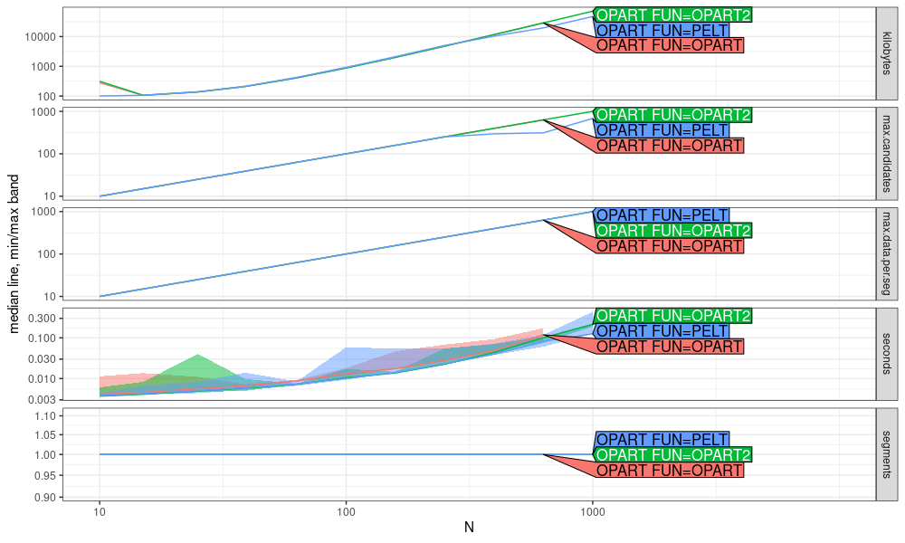
Above the resulting plot does not show much of a difference between
OPART and PELT, why? Remember in the previous section, we showed that
the number of candidates considered (and time complexity) depends on
the max size of the segments, which were 1000 in the simulation. In
the plot above we only go up to a data size of N=1000, so it is
normal that PELT looks the same as OPART (no pruning, constant/flat
data with no changes).
Another simulation
Below we simulate another data set with 10 data points per segment, so we should be able to see the difference between algorithms better.
set.seed(1)
more.mean.mat <- sim_means(N.segs=300, N.dim=2)
more.sim.mat <- sim_data(more.mean.mat, N.per.seg=10)
more_opart_vs_pelt <- atime_PELT(more.sim.mat, penalty=1)
plot(more_opart_vs_pelt)
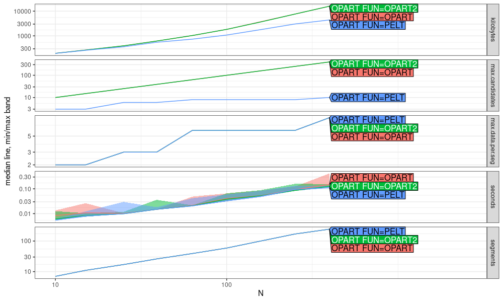
In the plot above, we can see some evidence of pruning.
- PELT memory usage in
kilobytesandmax.candidatesare smaller than OPART. - When the penalty is chosen correctly, we expect the max data per segment in this simulation to be 10, which we do not observe above, so the penalty could be modified (exercise for the reader).
- Computation time in
secondsfor PELT is about the same as OPART (bigger differences may be evident for larger data sizes N).
Conclusions
The OPART and PELT algorithms can be implemented using the cumsum trick in R. The PELT speedups are difficult to observe using pure R implementations, but it is possible to see the pruning by looking at the number of candidates considered. For even more pruning, and faster algorithms, the Functional Pruning technique of Maidstone et al (2017) can be used in the case of 1d data (not the case here, which used 2d data).
Session info
sessionInfo()
## R Under development (unstable) (2024-10-01 r87205)
## Platform: x86_64-pc-linux-gnu
## Running under: Ubuntu 22.04.5 LTS
##
## Matrix products: default
## BLAS:   /usr/lib/x86_64-linux-gnu/blas/libblas.so.3.10.0
## LAPACK: /usr/lib/x86_64-linux-gnu/lapack/liblapack.so.3.10.0
##
## locale:
##  [1] LC_CTYPE=fr_FR.UTF-8       LC_NUMERIC=C               LC_TIME=fr_FR.UTF-8        LC_COLLATE=fr_FR.UTF-8
##  [5] LC_MONETARY=fr_FR.UTF-8    LC_MESSAGES=fr_FR.UTF-8    LC_PAPER=fr_FR.UTF-8       LC_NAME=C
##  [9] LC_ADDRESS=C               LC_TELEPHONE=C             LC_MEASUREMENT=fr_FR.UTF-8 LC_IDENTIFICATION=C
##
## time zone: America/New_York
## tzcode source: system (glibc)
##
## attached base packages:
## [1] stats     graphics  utils     datasets  grDevices methods   base
##
## other attached packages:
## [1] ggplot2_3.5.1     data.table_1.16.2
##
## loaded via a namespace (and not attached):
##  [1] directlabels_2024.1.21 crayon_1.5.2           vctrs_0.6.5            knitr_1.47             cli_3.6.2
##  [6] xfun_0.45              rlang_1.1.3            highr_0.11             bench_1.1.3            generics_0.1.3
## [11] glue_1.7.0             labeling_0.4.3         colorspace_2.1-0       scales_1.3.0           fansi_1.0.6
## [16] quadprog_1.5-8         grid_4.5.0             evaluate_0.23          munsell_0.5.0          tibble_3.2.1
## [21] profmem_0.6.0          lifecycle_1.0.4        compiler_4.5.0         dplyr_1.1.4            pkgconfig_2.0.3
## [26] atime_2024.12.3        farver_2.1.1           lattice_0.22-6         R6_2.5.1               tidyselect_1.2.1
## [31] utf8_1.2.4             pillar_1.9.0           magrittr_2.0.3         tools_4.5.0            withr_3.0.0
## [36] gtable_0.3.4