Cross-validation with variable size train sets
The goal of this blog post is to explain how to use cross-validation,
as implemented in mlr3resampling::ResamplingVariableSizeTrain, for
determining how many samples are necessary for optimal prediction.
Simulated data
The code below creates data for simulated regression problems. First we define a vector of input values,
N <- 3000
abs.x <- 10
set.seed(1)
x.vec <- runif(N, -abs.x, abs.x)
str(x.vec)
## num [1:3000] -4.69 -2.56 1.46 8.16 -5.97 ...
Below we define a list of two true regression functions (tasks in mlr3 terminology) for our simulated data,
reg.pattern.list <- list(
  sin=sin,
  step=function(x)ifelse(x>0,1,0),
  linear=function(x)x/abs.x,
  quadratic=function(x)(x/abs.x)^2,
  constant=function(x)0)
The constant function represents a regression problem which can be solved by always predicting the mean value of outputs (featureless is the best possible learning algorithm). The other functions will be used to generate data with a pattern that will need to be learned. Below we use a for loop over these functions/tasks, to simulate the data which will be used as input to the learning algorithms:
library(data.table)
reg.task.list <- list()
reg.data.list <- list()
for(task_id in names(reg.pattern.list)){
  f <- reg.pattern.list[[task_id]]
  task.dt <- data.table(
    x=x.vec,
    y = f(x.vec)+rnorm(N,sd=0.5))
  reg.data.list[[task_id]] <- data.table(task_id, task.dt)
  reg.task.list[[task_id]] <- mlr3::TaskRegr$new(
    task_id, task.dt, target="y"
  )
}
(reg.data <- rbindlist(reg.data.list))
##         task_id          x           y
##          <char>      <num>       <num>
##     1:      sin -4.6898267  1.42476722
##     2:      sin -2.5575220 -1.01408083
##     3:      sin  1.4570673  1.44033043
##     4:      sin  8.1641558  0.48177556
##     5:      sin -5.9663614  0.58102619
##    ---
## 14996: constant -4.7724198 -0.24240068
## 14997: constant -7.8638912 -0.67924420
## 14998: constant -4.9248416  0.53996583
## 14999: constant -6.3819226  0.98559627
## 15000: constant  0.6277784  0.06898385
In the table above, the input is x, and the output is y. Below we visualize these data, with one task in each facet/panel:
if(require(animint2)){
  ggplot()+
    geom_point(aes(
      x, y),
      shape=1,
      data=reg.data)+
    facet_grid(. ~ task_id, labeller=label_both)
}
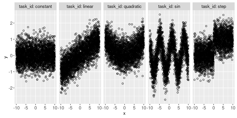
In the plot above we can see several different simulated data sets
(one in each panel). Note that the code above used the animint2
package, which provides interactive extensions to the static graphics
of the ggplot2 package (for an example see animint
gallery,
and source
code
in ResamplingVariableSizeTrainCV vignette).
Visualizing instance table
In the code below, we define a K-fold cross-validation experiment, with K=3 folds.
reg_size_cv <- mlr3resampling::ResamplingVariableSizeTrainCV$new()
reg_size_cv$param_set$values$train_sizes <- 20
reg_size_cv
## <ResamplingVariableSizeTrainCV> : Cross-Validation with variable size train sets
## * Iterations:
## * Instantiated: FALSE
## * Parameters:
## List of 4
##  $ folds         : int 3
##  $ min_train_data: int 10
##  $ random_seeds  : int 3
##  $ train_sizes   : int 20
In the output above we can see the parameters of the resampling object, all of which should be integer scalars:
foldsis the number of cross-validation folds.min_train_datais the minimum number of train data to consider.random_seedsis the number of random seeds, each of which determines a different random ordering of the train data. The random ordering determines which data are included in small train set sizes.train_sizesis the number of train set sizes, evenly spaced on a log scale, frommin_train_datato the max number of train data (determined byfolds).
Below we instantiate the resampling on one of the tasks:
reg_size_cv$instantiate(reg.task.list[["sin"]])
reg_size_cv$instance
## $iteration.dt
##      test.fold  seed train_size                             train                  test iteration
##          <int> <int>      <int>                            <list>                <list>     <int>
##   1:         1     1         10 1542,2786,1015, 209,1413,2290,...       2,3,4,6,7,8,...         1
##   2:         1     1         13 1542,2786,1015, 209,1413,2290,...       2,3,4,6,7,8,...         2
##   3:         1     1         17 1542,2786,1015, 209,1413,2290,...       2,3,4,6,7,8,...         3
##   4:         1     1         23 1542,2786,1015, 209,1413,2290,...       2,3,4,6,7,8,...         4
##   5:         1     1         31 1542,2786,1015, 209,1413,2290,...       2,3,4,6,7,8,...         5
##  ---
## 176:         3     3        656 1130,2594, 948,1451, 783,1024,...  1, 5, 9,12,15,16,...       176
## 177:         3     3        866 1130,2594, 948,1451, 783,1024,...  1, 5, 9,12,15,16,...       177
## 178:         3     3       1145 1130,2594, 948,1451, 783,1024,...  1, 5, 9,12,15,16,...       178
## 179:         3     3       1513 1130,2594, 948,1451, 783,1024,...  1, 5, 9,12,15,16,...       179
## 180:         3     3       2000 1130,2594, 948,1451, 783,1024,...  1, 5, 9,12,15,16,...       180
##
## $id.dt
##       row_id  fold
##        <int> <int>
##    1:      1     3
##    2:      2     1
##    3:      3     1
##    4:      4     1
##    5:      5     3
##   ---
## 2996:   2996     1
## 2997:   2997     1
## 2998:   2998     1
## 2999:   2999     2
## 3000:   3000     3
Above we see the instance, which need not be examined by the user, but for informational purposes, it contains the following data:
iteration.dthas one row for each train/test split,id.dthas one row for each data point.
Benchmark: computing test error
In the code below, we define two learners to compare,
(reg.learner.list <- list(
  if(requireNamespace("rpart"))mlr3::LearnerRegrRpart$new(),
  mlr3::LearnerRegrFeatureless$new()))
## [[1]]
## <LearnerRegrRpart:regr.rpart>: Regression Tree
## * Model: -
## * Parameters: xval=0
## * Packages: mlr3, rpart
## * Predict Types:  [response]
## * Feature Types: logical, integer, numeric, factor, ordered
## * Properties: importance, missings, selected_features, weights
##
## [[2]]
## <LearnerRegrFeatureless:regr.featureless>: Featureless Regression Learner
## * Model: -
## * Parameters: robust=FALSE
## * Packages: mlr3, stats
## * Predict Types:  [response], se
## * Feature Types: logical, integer, numeric, character, factor, ordered, POSIXct
## * Properties: featureless, importance, missings, selected_features
The code above defines
regr.rpart: Regression Tree learning algorithm, which should be able to learn any of the patterns (if there are enough data in the train set).regr.featureless: Featureless Regression learning algorithm, which should be optimal for the constant data, and can be used as a baseline in the other data. When the rpart learner gets smaller prediction error rates than featureless, then we know that it has learned some non-trivial relationship between inputs and outputs.
In the code below, we define the benchmark grid, which is all combinations of tasks, learners, and the one resampling method.
(reg.bench.grid <- mlr3::benchmark_grid(
  reg.task.list,
  reg.learner.list,
  reg_size_cv))
##          task          learner             resampling
##        <char>           <char>                 <char>
##  1:       sin       regr.rpart variable_size_train_cv
##  2:       sin regr.featureless variable_size_train_cv
##  3:      step       regr.rpart variable_size_train_cv
##  4:      step regr.featureless variable_size_train_cv
##  5:    linear       regr.rpart variable_size_train_cv
##  6:    linear regr.featureless variable_size_train_cv
##  7: quadratic       regr.rpart variable_size_train_cv
##  8: quadratic regr.featureless variable_size_train_cv
##  9:  constant       regr.rpart variable_size_train_cv
## 10:  constant regr.featureless variable_size_train_cv
In the code below, we execute the benchmark experiment (optionally in parallel using the multisession future plan).
if(require(future))plan("multisession")
lgr::get_logger("mlr3")$set_threshold("warn")
(reg.bench.result <- mlr3::benchmark(
  reg.bench.grid, store_models = TRUE))
## <BenchmarkResult> of 1800 rows with 10 resampling runs
##  nr   task_id       learner_id          resampling_id iters warnings errors
##   1       sin       regr.rpart variable_size_train_cv   180        0      0
##   2       sin regr.featureless variable_size_train_cv   180        0      0
##   3      step       regr.rpart variable_size_train_cv   180        0      0
##   4      step regr.featureless variable_size_train_cv   180        0      0
##   5    linear       regr.rpart variable_size_train_cv   180        0      0
##   6    linear regr.featureless variable_size_train_cv   180        0      0
##   7 quadratic       regr.rpart variable_size_train_cv   180        0      0
##   8 quadratic regr.featureless variable_size_train_cv   180        0      0
##   9  constant       regr.rpart variable_size_train_cv   180        0      0
##  10  constant regr.featureless variable_size_train_cv   180        0      0
The code below computes the test error for each split, and visualizes the information stored in the first row of the result:
reg.bench.score <- mlr3resampling::score(reg.bench.result)
reg.bench.score[1]
##    test.fold  seed train_size                             train            test iteration
##        <int> <int>      <int>                            <list>          <list>     <int>
## 1:         1     1         10 1542,2786,1015, 209,1413,2290,... 2,3,4,6,7,8,...         1
##                                   uhash    nr           task task_id                       learner learner_id
##                                  <char> <int>         <list>  <char>                        <list>     <char>
## 1: bd17f2fa-8999-4363-bfa2-c3f92ca3fc25     1 <TaskRegr:sin>     sin <LearnerRegrRpart:regr.rpart> regr.rpart
##                         resampling          resampling_id       prediction  regr.mse algorithm
##                             <list>                 <char>           <list>     <num>    <char>
## 1: <ResamplingVariableSizeTrainCV> variable_size_train_cv <PredictionRegr> 0.7323854     rpart
The output above contains all of the results related to a particular train/test split. In particular for our purposes, the interesting columns are:
test.foldis the cross-validation fold ID.seedis the random seed used to determine the train set order.train_sizeis the number of data in the train set.trainandtestare vectors of row numbers assigned to each set.iterationis an ID for the train/test split, for a particular learning algorithm and task. It is the row number ofiteration.dt(see instance above), which has one row for each unique combination oftest.fold,seed, andtrain_size.learneris the mlr3 learner object, which can be used to compute predictions on new data (including a grid of inputs, to show predictions in the visualization below).regr.mseis the mean squared error on the test set.algorithmis the name of the learning algorithm (same aslearner_idbut withoutregr.prefix).
The code below visualizes the resulting test accuracy numbers.
train_size_vec <- unique(reg.bench.score$train_size)
if(require(animint2)){
  ggplot()+
    scale_x_log10()+
    scale_y_log10(
      "Mean squared error on test set")+
    geom_line(aes(
      train_size, regr.mse,
      group=paste(algorithm, seed),
      color=algorithm),
      shape=1,
      data=reg.bench.score)+
    geom_point(aes(
      train_size, regr.mse, color=algorithm),
      shape=1,
      data=reg.bench.score)+
    facet_grid(
      test.fold~task_id,
      labeller=label_both,
      scales="free")
}
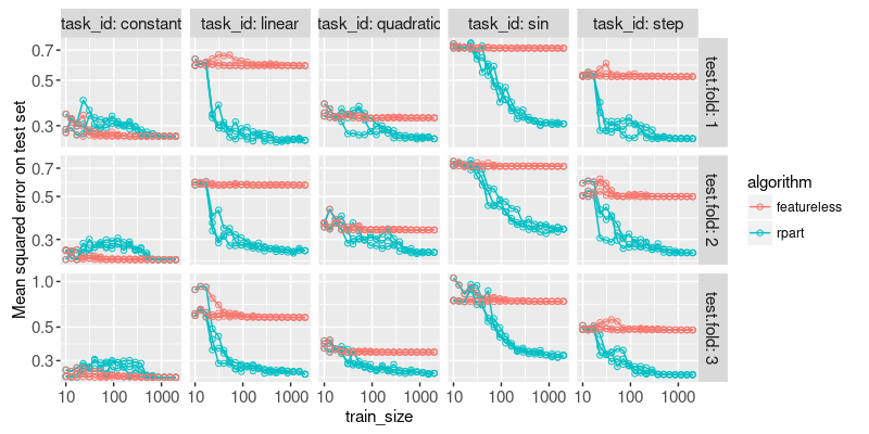
Above we plot the test error for each fold and train set size. There is a different panel for each task and test fold. Each line represents a random seed (ordering of data in train set), and each dot represents a specific train set size. So the plot above shows that some variation in test error, for a given test fold, is due to the random ordering of the train data.
Below we summarize each train set size, by taking the mean and standard deviation over each random seed.
reg.mean.dt <- dcast(
  reg.bench.score,
  task_id + train_size + test.fold + algorithm ~ .,
  list(mean, sd),
  value.var="regr.mse")
if(require(animint2)){
  ggplot()+
    scale_x_log10()+
    scale_y_log10(
      "Mean squared error on test set
(Mean +/- SD over 3 random orderings of train data)")+
    geom_ribbon(aes(
      train_size,
      ymin=regr.mse_mean-regr.mse_sd,
      ymax=regr.mse_mean+regr.mse_sd,
      fill=algorithm),
      alpha=0.5,
      data=reg.mean.dt)+
    geom_line(aes(
      train_size, regr.mse_mean, color=algorithm),
      shape=1,
      data=reg.mean.dt)+
    facet_grid(
      test.fold~task_id,
      labeller=label_both,
      scales="free")
}
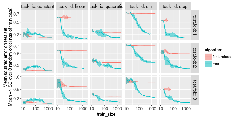
The plot above shows a line for the mean, and a ribbon for the standard deviation, over the three random seeds. It is clear from the plot above that
- in constant task, rpart sometimes overfits for intermediate sample sizes.
- in other tasks, rpart shows the expected test error curve, which decreases as train size increases.
- Test error curves are mostly flat when there are 1000 train samples, which indicates that gathering even more samples is not necessary.
Session info and citation
sessionInfo()
## R Under development (unstable) (2023-12-22 r85721)
## Platform: x86_64-pc-linux-gnu
## Running under: Ubuntu 22.04.3 LTS
##
## Matrix products: default
## BLAS:   /usr/lib/x86_64-linux-gnu/blas/libblas.so.3.10.0
## LAPACK: /usr/lib/x86_64-linux-gnu/lapack/liblapack.so.3.10.0
##
## locale:
##  [1] LC_CTYPE=fr_FR.UTF-8       LC_NUMERIC=C               LC_TIME=fr_FR.UTF-8        LC_COLLATE=fr_FR.UTF-8
##  [5] LC_MONETARY=fr_FR.UTF-8    LC_MESSAGES=fr_FR.UTF-8    LC_PAPER=fr_FR.UTF-8       LC_NAME=C
##  [9] LC_ADDRESS=C               LC_TELEPHONE=C             LC_MEASUREMENT=fr_FR.UTF-8 LC_IDENTIFICATION=C
##
## time zone: America/Phoenix
## tzcode source: system (glibc)
##
## attached base packages:
## [1] stats     graphics  utils     datasets  grDevices methods   base
##
## other attached packages:
## [1] mlr3_0.17.1         future_1.33.1       animint2_2023.11.21 data.table_1.14.99
##
## loaded via a namespace (and not attached):
##  [1] gtable_0.3.4              future.apply_1.11.1       compiler_4.4.0            highr_0.10
##  [5] crayon_1.5.2              rpart_4.1.23              Rcpp_1.0.11               stringr_1.5.1
##  [9] parallel_4.4.0            globals_0.16.2            scales_1.3.0              uuid_1.1-1
## [13] RhpcBLASctl_0.23-42       R6_2.5.1                  plyr_1.8.9                labeling_0.4.3
## [17] knitr_1.45                palmerpenguins_0.1.1      backports_1.4.1           checkmate_2.3.1
## [21] munsell_0.5.0             paradox_0.11.1            mlr3measures_0.5.0        rlang_1.1.2
## [25] stringi_1.8.3             lgr_0.4.4                 xfun_0.41                 mlr3misc_0.13.0
## [29] RJSONIO_1.3-1.9           cli_3.6.2                 magrittr_2.0.3            digest_0.6.33
## [33] grid_4.4.0                lifecycle_1.0.4           evaluate_0.23             glue_1.6.2
## [37] farver_2.1.1              listenv_0.9.0             codetools_0.2-19          parallelly_1.36.0
## [41] colorspace_2.1-0          reshape2_1.4.4            tools_4.4.0               mlr3resampling_2023.12.28
This blog post has been adapted from the ResamplingVariableSizeTrainCV vignette, but uses larger data.