Interpretable learning algorithms with built-in feature selection
Machine learning algorithms input a train data set, and output a prediction function. This post is about interpreting that prediction function, in terms of what input features in the data are used to compute predictions.
Introduction to model interpretation
Most machine learning algorithms output a prediction function that uses all of the input features in the train data set. In the special case of feature selection algorithms, a subset of input features is used in the prediction function. For example, the L1 regularized linear learning algorithm (R package glmnet) outputs a coefficient/weight vector with some values set to zero. We can therefore say that the model is interpretable in terms of the different input feature subsets:
- For the features with weights equal to zero, these features are completely ignored for the purposes of prediction (non-important subset of features).
- For the features with weights not equal to zero, these features are used to compute predictions (important subset of features).
In the next sections, we explain how to compute and interpret this algorithm using base R.
Data simulation
For the purposes of demonstrating the feature selection algorithms, we use the simulated data below:
N <- 3000
library(data.table)
set.seed(1)
n.features <- 9
(full.dt <- data.table()[
, paste0("x",1:n.features) := replicate(n.features, rnorm(N), simplify=FALSE)
][
, label := factor(ifelse(x1*2+x2-x3-x4*2+rnorm(N) < 0, "not spam", "spam"))
][])
##               x1         x2          x3         x4          x5         x6
##            <num>      <num>       <num>      <num>       <num>      <num>
##    1: -0.6264538  0.7391149 -0.61882708 -1.2171201 -0.93910663 -0.2139090
##    2:  0.1836433  0.3866087 -1.10942196 -0.9462293  1.39366493 -0.1067233
##    3: -0.8356286  1.2963972 -2.17033523  0.0914098  1.62581486 -0.4645893
##    4:  1.5952808 -0.8035584 -0.03130307  0.7013513  0.40900106 -0.6842725
##    5:  0.3295078 -1.6026257 -0.26039848  0.6734224 -0.09255856 -0.7908007
##   ---
## 2996: -0.1867578 -1.1915728 -0.98779143 -0.8189035 -0.27644611  0.5609876
## 2997: -0.2293598 -0.3313449  0.11387615  0.5540142 -0.57449307 -0.4323915
## 2998:  1.6301856  0.5007431  2.91226684 -0.4781837 -0.04188780 -0.3361756
## 2999: -2.1646714 -0.1734766  0.03440461 -0.7533612  0.05345084 -1.0955517
## 3000: -1.0777760  0.2572395  2.55225349 -0.3570393 -1.45209261  0.3467535
##               x7         x8         x9    label
##            <num>      <num>      <num>   <fctr>
##    1:  0.9514099  0.6010915  0.6756055     spam
##    2:  0.4570987 -2.7671158 -0.6491423     spam
##    3: -0.3586935  0.1815231 -1.4441087     spam
##    4: -1.0458614  2.2618871 -1.8403095     spam
##    5:  0.3075345  0.7119713  0.5150060 not spam
##   ---
## 2996: -1.5549427 -0.4318743  2.3534390     spam
## 2997:  0.4283458 -0.5406607  0.6931265 not spam
## 2998: -0.9993544  0.5154600  1.0578388     spam
## 2999:  0.4377104  0.7893972  0.7882958 not spam
## 3000: -1.7429542  0.4198874  0.2565586 not spam
table(full.dt$label)
##
## not spam     spam
##     1505     1495
We can imagine a spam filtering system, with training data for which each row in the table above represents a message which has been labeled as spam or not. In the table above, there are two sets of features:
x1tox4are used to define the outputlabel(and should be used in the best prediction function)- other features are random noise (should be ignored by the best prediction function)
In the next section, we run the L1 regularized linear learning algorithm on these data, along with another interpretable algorithm (decision tree).
mlr3 training
To use the mlr3 framework on our simulated data, we begin by converting the data table to a task in the code below,
(task.classif <- mlr3::TaskClassif$new(
  "simulated", full.dt, target="label"
)$set_col_roles("label", c("target", "stratum")))
## <TaskClassif:simulated> (3000 x 10)
## * Target: label
## * Properties: twoclass, strata
## * Features (9):
##   - dbl (9): x1, x2, x3, x4, x5, x6, x7, x8, x9
## * Strata: label
The output above shows that we have created a task named simulated, with target column named label, and with several features (x1 etc). The output also indicates the label column is used as a stratum, which means that when sampling, the proportion of each label in the subsample should match the proportion in the total data.
Below we create a resampling object that will vary the size of the train set,
size_cv <- mlr3resampling::ResamplingVariableSizeTrainCV$new()
size_cv$param_set$values$min_train_data <- 15
size_cv$param_set$values$random_seeds <- 4
size_cv
## <ResamplingVariableSizeTrainCV> : Cross-Validation with variable size train sets
## * Iterations:
## * Instantiated: FALSE
## * Parameters:
## List of 4
##  $ folds         : int 3
##  $ min_train_data: int 15
##  $ random_seeds  : int 4
##  $ train_sizes   : int 5
The output above indicates the resampling involves 3 cross-validation folds, 15 min train data (in smallest stratum), 4 random seeds, and 5 train sizes. All of these choices are arbitrary, and do not have a large effect on the end results. Exercise for the reader: play with these values, re-do the computations, and see if you get similar results. (you should!)
Below we define a list of learning algorithms, and note the
cv_glmnet learner internally uses cross-validation, with the given
number of folds (below 6), to select the optimal degree of L1
regularization (which maximizes prediction accuracy). Note that this
nfolds parameter controls the subtrain/validation split (used to
learn model complexity hyper-parameters), and is different from the
folds parameter of size_cv (which controls the train/test split,
useful for comparing prediction accuracy of learning algorithms).
cv_glmnet <- mlr3learners::LearnerClassifCVGlmnet$new()
cv_glmnet$param_set$values$nfolds <- 6
(learner.list <- list(
  cv_glmnet,
  mlr3::LearnerClassifRpart$new(),
  mlr3::LearnerClassifFeatureless$new()))
## [[1]]
## <LearnerClassifCVGlmnet:classif.cv_glmnet>: GLM with Elastic Net Regularization
## * Model: -
## * Parameters: nfolds=6
## * Packages: mlr3, mlr3learners, glmnet
## * Predict Types:  [response], prob
## * Feature Types: logical, integer, numeric
## * Properties: multiclass, selected_features, twoclass, weights
##
## [[2]]
## <LearnerClassifRpart:classif.rpart>: Classification Tree
## * Model: -
## * Parameters: xval=0
## * Packages: mlr3, rpart
## * Predict Types:  [response], prob
## * Feature Types: logical, integer, numeric, factor, ordered
## * Properties: importance, missings, multiclass, selected_features,
##   twoclass, weights
##
## [[3]]
## <LearnerClassifFeatureless:classif.featureless>: Featureless Classification Learner
## * Model: -
## * Parameters: method=mode
## * Packages: mlr3
## * Predict Types:  [response], prob
## * Feature Types: logical, integer, numeric, character, factor, ordered,
##   POSIXct
## * Properties: featureless, importance, missings, multiclass,
##   selected_features, twoclass
The output above shows a list of three learning algorithms.
cv_glmnetis the L1 regularized linear model, which will set some weights to zero (selecting the other features).rpartis another learning algorithm with built-in feature selection, which will be discussed below.featurelessis a baseline learning algorithm which always predicts the most frequent label in the train set. This should always be run for comparison with the real learning algorithms (which will be more accurate if they have learned some non-trivial relationship between inputs/features and output/target).
Below we define a benchmark grid, which combines our task, with learners, and the resampling,
(bench.grid <- mlr3::benchmark_grid(
  task.classif,
  learner.list,
  size_cv))
##         task             learner             resampling
##       <char>              <char>                 <char>
## 1: simulated   classif.cv_glmnet variable_size_train_cv
## 2: simulated       classif.rpart variable_size_train_cv
## 3: simulated classif.featureless variable_size_train_cv
The output above is a table with one row for each combination of task, learner, and resampling.
Below we first define a future plan to do the computations in parallel, then set log threshold to reduce output, then compute the benchmark result.
if(require(future))plan("multisession")
lgr::get_logger("mlr3")$set_threshold("warn")
(bench.result <- mlr3::benchmark(
  bench.grid, store_models = TRUE))
## Warning: from glmnet C++ code (error code -96); Convergence for 96th lambda
## value not reached after maxit=100000 iterations; solutions for larger lambdas
## returned
## <BenchmarkResult> of 180 rows with 3 resampling runs
##  nr   task_id          learner_id          resampling_id iters warnings errors
##   1 simulated   classif.cv_glmnet variable_size_train_cv    60        0      0
##   2 simulated       classif.rpart variable_size_train_cv    60        0      0
##   3 simulated classif.featureless variable_size_train_cv    60        0      0
The output above shows the number of resampling iterations computed.
interpreting prediction error rates on test set
The code below computes scores (test error), for each resampling iteration.
bench.score <- mlr3resampling::score(bench.result)
bench.score[1]
##    test.fold  seed small_stratum_size train_size_i train_size
##        <int> <int>              <int>        <int>      <int>
## 1:         1     1                 15            1         30
##                                train                  test iteration
##                               <list>                <list>     <int>
## 1: 2071,1092, 723,2654,  49,2834,...  3,11,20,21,26,34,...         1
##    train_min_size                                uhash    nr
##             <int>                               <char> <int>
## 1:             30 a3a36ae1-132b-4432-83f6-e3ee3536960d     1
##                       task   task_id                                    learner
##                     <list>    <char>                                     <list>
## 1: <TaskClassif:simulated> simulated <LearnerClassifCVGlmnet:classif.cv_glmnet>
##           learner_id                      resampling          resampling_id
##               <char>                          <list>                 <char>
## 1: classif.cv_glmnet <ResamplingVariableSizeTrainCV> variable_size_train_cv
##             prediction classif.ce algorithm
##                 <list>      <num>    <char>
## 1: <PredictionClassif>  0.2557443 cv_glmnet
The output above shows the result of one resampling iteration. Important columns include
train_size, number of samples in train set.train_size_i, train set sample size iteration number.train_min_size, min oftrain_sizeover all values oftrain_size_i, useful for plotting because there may be slight variations intrain_sizebetween folds.classif.ce, test error (mis-classification rate).algorithm, learning algorithm.test.fold, test fold number in cross-validation.seed, random seed used to determine sampling order through train set.
Below we plot the results,
train_min_size_vec <- unique(bench.score[["train_min_size"]])
library(animint2)
ggplot()+
  scale_x_log10(breaks=train_min_size_vec)+
  scale_y_continuous(
    "Classification error on test set")+
  geom_line(aes(
    train_min_size, classif.ce,
    group=paste(algorithm, seed),
    color=algorithm),
    shape=1,
    data=bench.score)+
  geom_point(aes(
    train_min_size, classif.ce, color=algorithm),
    shape=1,
    data=bench.score)+
  facet_grid(
    test.fold~task_id,
    labeller=label_both)
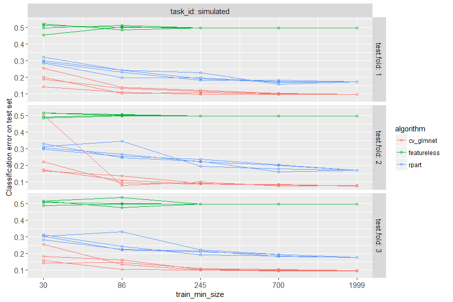
The figure above has a panel for each test fold in cross-validation.
There is a line for each algorithm, and for each random seed. The
plot is test error as a function of train size, so we can see how many
samples are required to learn a reasonable prediction function. It is
clear that a small number of samples (20) is not sufficient for either
learning algorithm, and a large number of samples (2000) is enough to
learn good predictions (with significantly smaller error rate than
featureless). Interestingly, the linear model is actually more
accurate than the decision tree, for intermediate and large data sizes.
This makes sense, because label was defined using a linear function.
interpreting linear model
In this section we show how to interpret the learned linear models, in terms of the weights. First we consider the subset of score table rows which correspond to the linear model. Then we loop over each row, computing the weight vector learned in each train/test split. We then combine the learned weights together in a single data table.
library(glmnet)
glmnet.score <- bench.score[algorithm=="cv_glmnet"]
weight.dt.list <- list()
levs <- grep("^x", names(full.dt), value=TRUE)
for(score.i in 1:nrow(glmnet.score)){
  score.row <- glmnet.score[score.i]
  fit <- score.row$learner[[1]]$model
  weight.mat <- coef(fit)[-1,]
  weight.dt.list[[score.i]] <- score.row[, .(
    test.fold, seed, train_min_size,
    weight=as.numeric(weight.mat),
    variable=factor(names(weight.mat), levs))]
}
(weight.dt <- rbindlist(weight.dt.list))
##      test.fold  seed train_min_size      weight variable
##          <int> <int>          <int>       <num>   <fctr>
##   1:         1     1             30 -1.80753945       x1
##   2:         1     1             30 -0.12733950       x2
##   3:         1     1             30  0.21719221       x3
##   4:         1     1             30  0.09392049       x4
##   5:         1     1             30  0.00000000       x5
##  ---
## 536:         3     4           1999  0.00000000       x5
## 537:         3     4           1999  0.00000000       x6
## 538:         3     4           1999  0.00000000       x7
## 539:         3     4           1999  0.00000000       x8
## 540:         3     4           1999  0.00000000       x9
The output above shows one row for each weight learned in each train/test split. Most weights are zero (not used for prediction), due to L1 regularization. We use the code below to visualize these weights.
weight.non.zero <- weight.dt[weight!=0]
ggplot()+
  facet_grid(test.fold ~ seed, labeller=label_both)+
  scale_y_discrete(breaks=levs,drop=FALSE)+
  geom_tile(aes(
    train_min_size, variable, fill=weight),
    data=weight.non.zero)+
  scale_fill_gradient2()+
  scale_x_log10(breaks=train_min_size_vec)+
  theme(axis.text.x=element_text(angle=60, hjust=1))
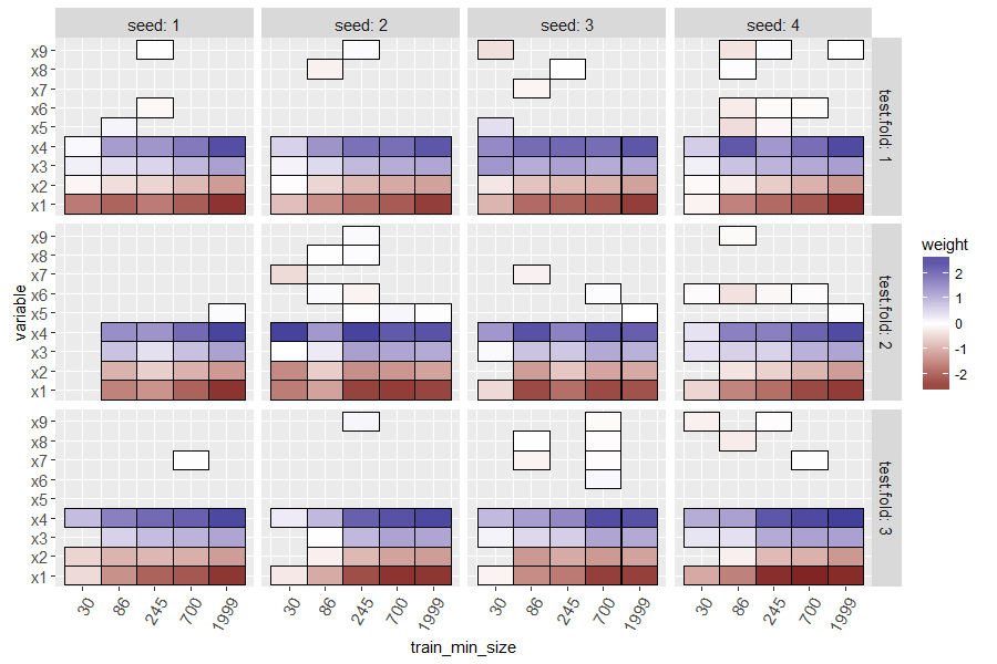
The heat map above shows a tile for each seed, train size, test fold, and variable. Missing tiles (grey background) indicate zero weights (not used for prediction. Recall that in our simulated data, there was only one signal feature (x0) and the others are noise that should be ignored. It is clear that at small train sizes, there are some false positive non-zero weights, and there are also false negatives (weight for x0 should not be zero). For large train sizes, the L1 regularization does a good job of selecting only the important variable (x0 has negative weight, and others have zero weight).
Typically positive weights mean that larger feature values mean more likelihood of being classified as positive (and negative weights/smaller feature values would be the opposite), but mlr3 seems to invert the glmnet weights, which I reported as an issue.
Another method which I typically use for interpreting L1 regularized linear models involves counting folds/splits with non-zero weight, for each variable. To do that we can use the code below,
ggplot()+
  scale_y_discrete(breaks=levs,drop=FALSE)+
  theme_bw()+
  geom_vline(xintercept=0, color="grey50")+
  geom_point(aes(
    weight, variable),
    shape=1,
    data=weight.non.zero)+
  facet_grid(seed ~ train_min_size, labeller=label_both)
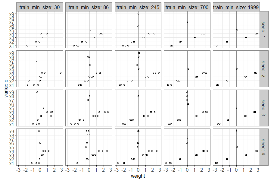
The plot above shows a point for each non-zero linear model weight,
with one panel for each seed and train size. There is a vertical grey
line to emphasize a weight value of zero. It is clear that large train
sizes result in three points/folds with non-zero weights, for the
signal feature x0, and zero weights for the other noise features.
We can also use the number of folds with non zero weights as a metric for variable importance, as we compute in the code below.
(one.panel <- weight.non.zero[
  train_min_size==86 & seed==2
][
, non.zero.folds := .N, by=variable
])
var.ord.dt <- one.panel[, .(
  mean.weight=mean(weight)
), by=.(variable, non.zero.folds)
][order(-non.zero.folds, -abs(mean.weight))]
var.ord.levs <- paste(var.ord.dt$variable)
one.panel[, Variable := factor(variable, var.ord.levs)]
ggplot()+
  theme_bw()+
  geom_vline(xintercept=0, color="grey50")+
  geom_point(aes(
    weight, Variable),
    shape=1,
    data=one.panel)+
  facet_grid(non.zero.folds ~ ., scales="free", space="free")
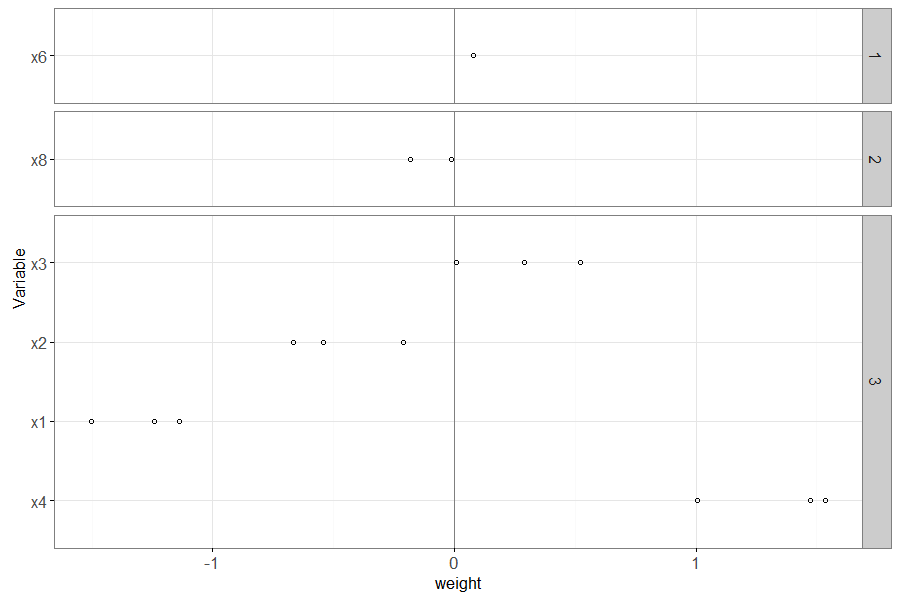
The plot above has a panel for each value of non.zero.folds – the
variables that appear in the larger panel numbers are more important
(have non-zero weights in more folds).
Also, within each panel, the most important variables (with largest absolute weight) appear near the bottom.
interpreting decision tree
Another machine learning algorithm with built-in feature selection is the decision tree, which we can interpret using the code below.
rpart.score <- bench.score[algorithm=="rpart"]
decision.dt.list <- list()
for(rpart.i in 1:nrow(rpart.score)){
  rpart.row <- rpart.score[rpart.i]
  rfit <- rpart.row$learner[[1]]$model
  decision.dt.list[[rpart.i]] <- rpart.row[, .(
    test.fold, seed, train_min_size,
    rfit$frame
  )][var!="<leaf>"]
}
(decision.dt <- rbindlist(decision.dt.list))
##      test.fold  seed train_min_size    var     n    wt   dev  yval complexity
##          <int> <int>          <int> <char> <int> <num> <num> <num>      <num>
##   1:         1     1             30     x1    30    30    15     1 0.80000000
##   2:         1     1             86     x1    86    86    43     1 0.58139535
##   3:         1     1             86     x4    59    59    17     1 0.11627907
##   4:         1     1             86     x2    21    21     8     2 0.09302326
##   5:         1     1            245     x1   245   245   122     1 0.45901639
##  ---
## 365:         3     4           1999     x4   162   162    77     1 0.01955868
## 366:         3     4           1999     x4   912   912   232     2 0.04012036
## 367:         3     4           1999     x1   313   313   139     1 0.04012036
## 368:         3     4           1999     x2   238   238    79     1 0.02006018
## 369:         3     4           1999     x4    82    82    31     2 0.01203611
##      ncompete nsurrogate yval2.V1 yval2.V2 yval2.V3  yval2.V4  yval2.V5
##         <int>      <int>    <num>    <num>    <num>     <num>     <num>
##   1:        4          5        1       15       15 0.5000000 0.5000000
##   2:        4          3        1       43       43 0.5000000 0.5000000
##   3:        4          5        1       42       17 0.7118644 0.2881356
##   4:        4          5        2        8       13 0.3809524 0.6190476
##   5:        4          5        1      123      122 0.5020408 0.4979592
##  ---
## 365:        4          5        1       85       77 0.5246914 0.4753086
## 366:        4          5        2      232      680 0.2543860 0.7456140
## 367:        4          3        1      174      139 0.5559105 0.4440895
## 368:        4          5        1      159       79 0.6680672 0.3319328
## 369:        4          1        2       31       51 0.3780488 0.6219512
##      yval2.nodeprob
##               <num>
##   1:     1.00000000
##   2:     1.00000000
##   3:     0.68604651
##   4:     0.24418605
##   5:     1.00000000
##  ---
## 365:     0.08095952
## 366:     0.45577211
## 367:     0.15642179
## 368:     0.11894053
## 369:     0.04097951
The code above examines the splits which are used in each decision tree, and outputs a table above with one row per split used. The code below computes a table with one row per variable, with additional columns splits and samples to measure importance.
(var.dt <- decision.dt[, .(
  samples=sum(n),
  splits=.N
), by=.(test.fold, seed, train_min_size, variable=factor(var, levs))])
##      test.fold  seed train_min_size variable samples splits
##          <int> <int>          <int>   <fctr>   <int>  <int>
##   1:         1     1             30       x1      30      1
##   2:         1     1             86       x1      86      1
##   3:         1     1             86       x4      59      1
##   4:         1     1             86       x2      21      1
##   5:         1     1            245       x1     335      3
##  ---
## 177:         3     4            700       x2     140      2
## 178:         3     4           1999       x1    2836      3
## 179:         3     4           1999       x4    2245      4
## 180:         3     4           1999       x3     348      1
## 181:         3     4           1999       x2     238      1
The code below computes the proportion of samples used in each split, which is another measure of importance.
var.dt[
, split.sample.prop := samples/sum(samples)
, by=.(test.fold, seed, train_min_size)
][]
##      test.fold  seed train_min_size variable samples splits split.sample.prop
##          <int> <int>          <int>   <fctr>   <int>  <int>             <num>
##   1:         1     1             30       x1      30      1        1.00000000
##   2:         1     1             86       x1      86      1        0.51807229
##   3:         1     1             86       x4      59      1        0.35542169
##   4:         1     1             86       x2      21      1        0.12650602
##   5:         1     1            245       x1     335      3        0.45827633
##  ---
## 177:         3     4            700       x2     140      2        0.06068487
## 178:         3     4           1999       x1    2836      3        0.50044115
## 179:         3     4           1999       x4    2245      4        0.39615317
## 180:         3     4           1999       x3     348      1        0.06140815
## 181:         3     4           1999       x2     238      1        0.04199753
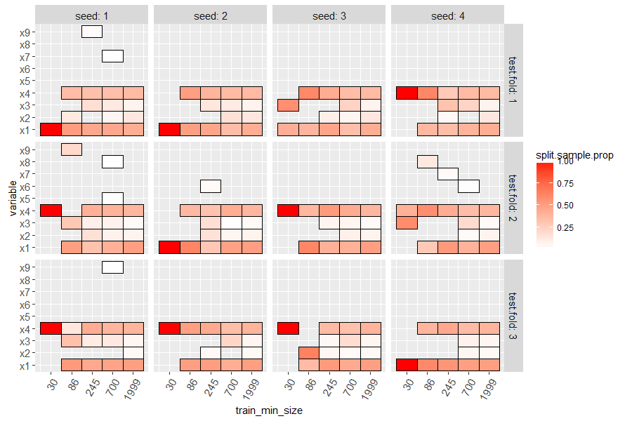
The code below makes a heatmap with a tile for each variable which was
used in at least one split of the learned decision tree. Larger values
of split.sample.prop (more red) indicate variables which are more
important (used with more samples).
ggplot()+
  facet_grid(test.fold ~ seed, labeller=label_both)+
  geom_tile(aes(
    train_min_size, variable, fill=split.sample.prop),
    data=var.dt)+
  scale_y_discrete(breaks=levs,drop=FALSE)+
  scale_fill_gradient(low="white", high="red")+
  scale_x_log10(breaks=train_min_size_vec)+
  theme(axis.text.x=element_text(angle=60, hjust=1))
Finally we make an analogous plot to the linear model below.
(one.rpart <- var.dt[
  train_min_size==700 & seed==4
][
, non.zero.folds := .N, by=variable
])
rpart.ord.dt <- one.rpart[, .(
  mean.prop=mean(split.sample.prop)
), by=.(variable, non.zero.folds)
][order(-non.zero.folds, -mean.prop)]
rpart.ord.levs <- paste(rpart.ord.dt$variable)
one.rpart[, Variable := factor(variable, rpart.ord.levs)]
ggplot()+
  theme_bw()+
  geom_point(aes(
    split.sample.prop, Variable),
    shape=1,
    data=one.rpart)+
  facet_grid(non.zero.folds ~ ., scales="free", space="free")
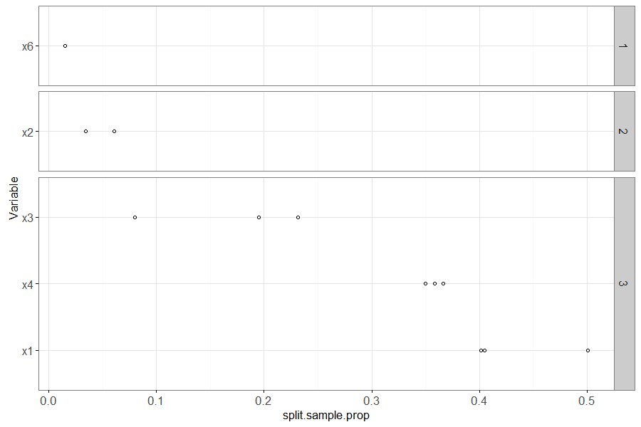
The plot above shows variable importance in the learned rpart model (decision tree). It shows the mean proportion of samples used in each split of the decision tree, for each variable, with one point for each fold in which that variable appeared in the decision tree (un-used variables do not appear in the plot). The number in the panel shows the number of folds for which this variable was used in the decision tree. The most important variables are sorted to the bottom of the plot (and x1 and x4 correctly appear there).
Conclusions
We have shown how to interpret two kinds of feature selection machine learning algorithms, L1 regularized linear models and decision trees, after having learned them using the mlr3 framework in R.
Session info
sessionInfo()
## R Under development (unstable) (2024-01-23 r85822 ucrt)
## Platform: x86_64-w64-mingw32/x64
## Running under: Windows 10 x64 (build 19045)
##
## Matrix products: default
##
##
## locale:
## [1] LC_COLLATE=English_United States.utf8
## [2] LC_CTYPE=English_United States.utf8
## [3] LC_MONETARY=English_United States.utf8
## [4] LC_NUMERIC=C
## [5] LC_TIME=English_United States.utf8
##
## time zone: America/Phoenix
## tzcode source: internal
##
## attached base packages:
## [1] stats     graphics  grDevices utils     datasets  methods   base
##
## other attached packages:
## [1] glmnet_4.1-8       Matrix_1.6-5       animint2_2024.1.24 future_1.33.2
## [5] data.table_1.15.99
##
## loaded via a namespace (and not attached):
##  [1] gtable_0.3.4             future.apply_1.11.2      highr_0.10
##  [4] compiler_4.4.0           BiocManager_1.30.22      crayon_1.5.2
##  [7] rpart_4.1.23             Rcpp_1.0.12              stringr_1.5.1
## [10] parallel_4.4.0           splines_4.4.0            globals_0.16.3
## [13] scales_1.3.0             uuid_1.2-0               RhpcBLASctl_0.23-42
## [16] lattice_0.22-5           R6_2.5.1                 plyr_1.8.9
## [19] labeling_0.4.3           shape_1.4.6.1            knitr_1.46
## [22] iterators_1.0.14         palmerpenguins_0.1.1     backports_1.4.1
## [25] checkmate_2.3.1          munsell_0.5.1            paradox_0.11.1
## [28] mlr3measures_0.5.0       rlang_1.1.3              stringi_1.8.3
## [31] lgr_0.4.4                xfun_0.43                mlr3_0.18.0
## [34] mlr3misc_0.15.0          RJSONIO_1.3-1.9          cli_3.6.2
## [37] magrittr_2.0.3           foreach_1.5.2            digest_0.6.34
## [40] grid_4.4.0               mlr3learners_0.5.8       lifecycle_1.0.4
## [43] evaluate_0.23            glue_1.7.0               farver_2.1.1
## [46] listenv_0.9.1            codetools_0.2-19         survival_3.5-7
## [49] parallelly_1.37.1        colorspace_2.1-0         reshape2_1.4.4
## [52] tools_4.4.0              mlr3resampling_2024.4.14