Partial matching on data frame row names
The goal of this blog post is to use my atime R package to explore the time it takes to subset a data frame using row names, and compare to other ways of doing that.
Introductory email to R-devel
Hilmar Berger wrote an email to the R-devel email list on 11 Dec 2023: “I have a different issue with the partial matching, in particular its performance when used on large data frames or more specifically, with large queries matched against its row names. I came across a case where I wanted to extract data from a large table (approx 1M rows) using an index which matched only about 50% to the row names, i.e. about 50% row name hits and 50% misses. What was unexpected is that in this case was that [.data.frame was hanging for a long time (I waited about 10 minutes and then restarted R). Also, this cannot be interrupted in interactive mode.”
The code and results he shared are below,
ids <- paste0("cg", sprintf("%06d",0:(1e6-1)))
d1 <- data.frame(row.names=ids, v=1:(1e6) )

q1 <- sample(ids, 1e6, replace=F)
system.time({r <- d1[q1,,drop=F]})
#   user  system elapsed
#  0.464   0.000   0.465

# those will hang a long time, I stopped R after 10 minutes
q2 <- c(q1[1:5e5], gsub("cg", "ct", q1[(5e5+1):1e6]) )
system.time({r <- d1[q2,,drop=F]})

# same here
q3 <- c(q1[1:5e5], rep("FOO",5e5) )
system.time({r <- d1[q3,,drop=F]})
He then observed, “It seems that the penalty of partial matching the
non-hits across the whole row name vector is not negligible any more
with large tables and queries, compared to small and medium tables. I
checked and pmatch(q2, rownames(d1) [sic] is equally slow. Is there a
chance to a) document this in the help page (“with large
indexes/tables use match()”) or even better b) add an exact flag to
[.data.frame ?”
Running his code
ids <- paste0("cg", sprintf("%06d",0:(1e6-1)))
d1 <- data.frame(row.names=ids, v=1:(1e6) )
head(d1)
##          v
## cg000000 1
## cg000001 2
## cg000002 3
## cg000003 4
## cg000004 5
## cg000005 6
q1 <- sample(ids, 1e6, replace=F)
head(q1)
## [1] "cg187369" "cg407503" "cg964183" "cg595617" "cg628810" "cg979990"
The output above shows that the data frame d1 has row names and a
single column, and the query q1 consists of several row names in
random order.
system.time({r <- d1[q1,,drop=F]})
## utilisateur     système      écoulé
##       1.784       0.000       1.863
head(r)
##               v
## cg187369 187370
## cg407503 407504
## cg964183 964184
## cg595617 595618
## cg628810 628811
## cg979990 979991
The times in the output above are a bit slower than in his original email, probably because my 15 year old Mac laptop is older than his computer.
The code below apparently hangs R, so I will not execute it:
# those will hang a long time, I stopped R after 10 minutes
q2 <- c(q1[1:5e5], gsub("cg", "ct", q1[(5e5+1):1e6]) )
system.time({r <- d1[q2,,drop=F]})
# same here
q3 <- c(q1[1:5e5], rep("FOO",5e5) )
system.time({r <- d1[q3,,drop=F]})
Instead I translate it to a smaller N below:
N <- 1e4L
N.v <- 1:N
N.ids <- paste0("cg", sprintf("%06d",N.v-1))
N.d <- data.frame(row.names=N.ids, N.v)
head(N.d)
##          N.v
## cg000000   1
## cg000001   2
## cg000002   3
## cg000003   4
## cg000004   5
## cg000005   6
N.half <- as.integer(N/2)
N.q1 <- sample(N.ids, N, replace=F)
N.q2 <- c(N.q1[1:N.half], gsub("cg", "ct", N.q1[(N.half+1):N]) )
N.q3 <- c(N.q1[1:N.half], rep("FOO",N.half) )
library(data.table)
data.table(N.q1, N.q2)
##            N.q1     N.q2
##     1: cg003793 cg003793
##     2: cg004553 cg004553
##     3: cg000282 cg000282
##     4: cg009698 cg009698
##     5: cg002789 cg002789
##    ---
##  9996: cg003522 ct003522
##  9997: cg006923 ct006923
##  9998: cg008929 ct008929
##  9999: cg004707 ct004707
## 10000: cg002940 ct002940
system.time({r1 <- N.d[N.q1,,drop=F]})
## utilisateur     système      écoulé
##       0.008       0.000       0.009
system.time({r2 <- N.d[N.q2,,drop=F]})
## utilisateur     système      écoulé
##       0.703       0.004       0.709
system.time({r3 <- N.d[N.q3,,drop=F]})
## utilisateur     système      écoulé
##       0.704       0.004       0.709
The output above suggests that the second and third queries (which contain half non-matching names) are about 100x slower than the first (which contains all matching names).
translating to atime code
In this section we translate the above example to use my atime
package, so we can easily see the asymptotic time complexity. To use
atime, we first need to make the code a function of some data size N,
which we already did in the previous section. Then we need to separate
the setup code (which constructs the data of size N) from the timing
code (which we want to measure), and that is actually already done too
(timing code is in system.time above). So the atime code is below:
atime.result <- atime::atime(
  N=10^seq(1, 6, by=0.5),
  setup={
    N.v <- 1:N
    N.ids <- paste0("cg", sprintf("%06d",N.v-1))
    N.d <- data.frame(row.names=N.ids, N.v)
    N.half <- as.integer(N/2)
    N.q1 <- sample(N.ids, N, replace=F)
    N.q2 <- c(N.q1[1:N.half], gsub("cg", "ct", N.q1[(N.half+1):N]) )
    N.q3 <- c(N.q1[1:N.half], rep("FOO",N.half) )
  },
  all.match=N.d[N.q1,,drop=F],
  half.no.match.ct=N.d[N.q2,,drop=F],
  half.no.match.FOO=N.d[N.q3,,drop=F])
plot(atime.result)
## Warning: Transformation introduced infinite values in continuous y-axis
## Transformation introduced infinite values in continuous y-axis
## Transformation introduced infinite values in continuous y-axis
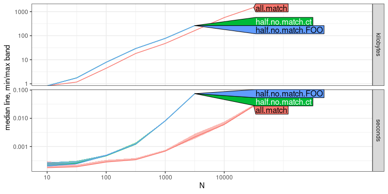
The output above is a plot of memory (kilobytes) and time (seconds)
usage as a function of data size N. The top panel (kilobytes) shows
that all three methods have the same asymptotic slope, which implies
that they are only different by constant factors, in terms of
memory. The bottom panel (seconds) shows that all.match has a
smaller slope than the other two, which implies that it has a faster
asymptotic time complexity. To determine the complexity classes, we
can use the code below:
atime.refs <- atime::references_best(atime.result)
plot(atime.refs)
## Warning: Transformation introduced infinite values in continuous y-axis
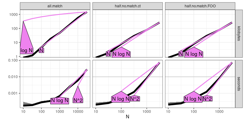
The output above is similar to the previous plot, but rather than show each of the three expressions in different colors, it shows each in a panel (from left to right). It additionally shows asymptotic reference lines, so we can see that the half match expressions are quadratic, whereas the all match expression is definitely sub-quadratic (seems to be log-linear, which implies a sort operation).
Comparison
Hilmar wrote in his original email, “I have seen that others have
discussed the partial matching behaviour of data.frame[idx,] in the
past, in particular with respect to unexpected results sets. I am
aware of the fact that one can work around this using either match()
or switching to tibble/data.table or similar altogether.”
Below we implement these work arounds:
workaround.result <- atime::atime(
  N=10^seq(1, 7, by=0.5),
  setup={
    N.v <- 1:N
    N.ids <- paste0("cg", sprintf("%06d",N.v-1))
    N.d <- data.frame(row.names=N.ids, N.v)
    N.half <- as.integer(N/2)
    matching.str <- sample(N.ids, N, replace=F)
    half.no.match <- c(matching.str[1:N.half], rep("FOO",N.half) )
    N.dt <- data.table(N.d, name=N.ids, key="name")
    N.tib <- tibble::tibble(N.d)
  },
  all.match=N.d[matching.str,,drop=F],
  half.no.match=N.d[half.no.match,,drop=F],
  match=N.d[match(half.no.match, rownames(N.d)),,drop=F],
  data.table=N.dt[half.no.match],
  tibble=N.tib[half.no.match,],
  seconds.limit=1)
plot(workaround.result)
## Warning: Transformation introduced infinite values in continuous y-axis
## Transformation introduced infinite values in continuous y-axis
## Transformation introduced infinite values in continuous y-axis
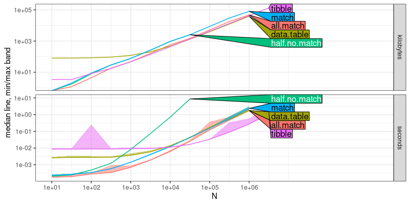
The output above shows that the half.no.match method has
asypmptotically larger slope than the other four methods, which
indicates the work-arounds are asymptotically faster, as expected.
workaround.refs <- atime::references_best(workaround.result)
plot(workaround.refs)
## Warning: Transformation introduced infinite values in continuous y-axis
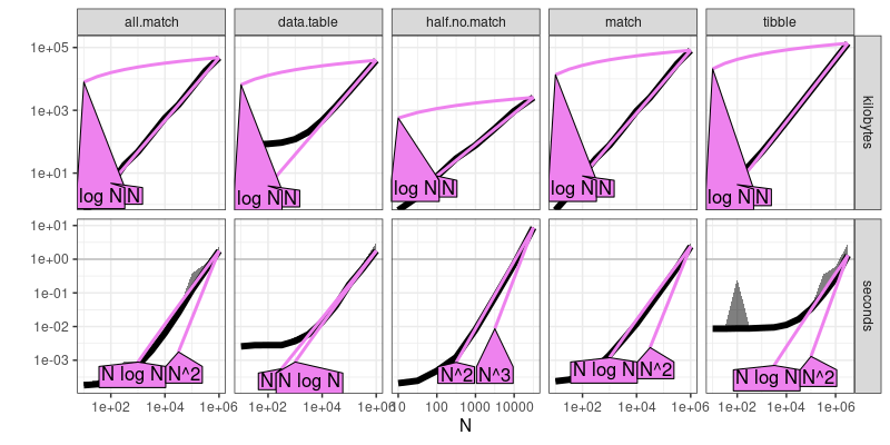
The output above shows that the work-arounds are all asyptotically sub-quadratic time, as expected.
Comparison with patch
Ivan Krylov proposed a patch on
R-devel,
which adds a new argument pmatch.rows that defaults to TRUE (for
backwards compatibility) but can be set to FALSE (to save time). Below
we use atime to show that this patch works for decreasing the
asymptotic time complexity,
patch.result <- atime::atime(
  N=10^seq(1, 7, by=0.5),
  setup={
    N.v <- 1:N
    N.ids <- paste0("cg", sprintf("%06d",N.v-1))
    N.d <- data.frame(row.names=N.ids, N.v)
    N.half <- as.integer(N/2)
    matching.str <- sample(N.ids, N, replace=F)
    half.no.match <- c(matching.str[1:N.half], rep("FOO",N.half) )
  },
  all.match=N.d[matching.str,,drop=F],
  half.no.match=N.d[half.no.match,,drop=F],
  "pmatch.rows=F"=N.d[half.no.match,,drop=F,pmatch.rows=F])
plot(patch.result)
## Warning: Transformation introduced infinite values in continuous y-axis
## Transformation introduced infinite values in continuous y-axis
## Transformation introduced infinite values in continuous y-axis
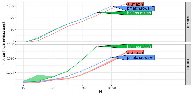
Note the code above will only run if you apply the patch to the R
source code, and re-compile/install R. The result above shows that
half.no.match time has a larger asymptotic slope than the other two
methods, which indicates that it is asymptotically slower. Below we
add asymptotic reference lines:
patch.refs <- atime::references_best(patch.result)
plot(patch.refs)
## Warning: Transformation introduced infinite values in continuous y-axis
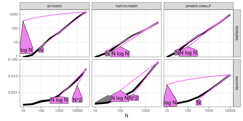
The output above shows that half.no.match is quadratic time, whereas
the other two methods are sub-quadratic.
Conclusion
The atime package is useful for comparing asymptotic time and memory
usage of various R expressions. In this post, we saw how it can be
used to show the quadratic time complexity of the base R data frame
row subset method, when there are a linear number of queries which do
not match. We also saw how various work-arounds are all sub-quadratic
time (pmatch, tibble, data.table, proposed pmatch.rows patch).
Session/version info
Note that the session info below says that R-devel was used, and in
fact it was a
patched
version of R-devel. If you do not want to apply the patch yourself,
you can clone my fork of
r-svn,
and checkout the df-partial-match-optional branch:
git clone https://github.com/tdhock/r-svn
cd r-svn
git checkout df-partial-match-optional
sed -i.bak 's|$(GIT) svn info|./.github/workflows/svn-info.sh|' Makefile.in
./.github/workflows/wget-recommended.sh
./.github/workflows/svn-info.sh
CFLAGS=-march=core2 CPPFLAGS=-march=core2 ./configure --prefix=$HOME --with-cairo --with-blas --with-lapack --enable-R-shlib --with-valgrind-instrumentation=2 --enable-memory-profiling
make
make install
sessionInfo()
## R Under development (unstable) (2022-03-22 r81960)
## Platform: x86_64-pc-linux-gnu (64-bit)
## Running under: Ubuntu 22.04.3 LTS
##
## Matrix products: default
## BLAS:   /usr/lib/x86_64-linux-gnu/blas/libblas.so.3.10.0
## LAPACK: /usr/lib/x86_64-linux-gnu/lapack/liblapack.so.3.10.0
##
## locale:
##  [1] LC_CTYPE=fr_FR.UTF-8       LC_NUMERIC=C               LC_TIME=fr_FR.UTF-8        LC_COLLATE=fr_FR.UTF-8
##  [5] LC_MONETARY=fr_FR.UTF-8    LC_MESSAGES=fr_FR.UTF-8    LC_PAPER=fr_FR.UTF-8       LC_NAME=C
##  [9] LC_ADDRESS=C               LC_TELEPHONE=C             LC_MEASUREMENT=fr_FR.UTF-8 LC_IDENTIFICATION=C
##
## attached base packages:
## [1] stats     graphics  utils     datasets  grDevices methods   base
##
## other attached packages:
## [1] data.table_1.14.10
##
## loaded via a namespace (and not attached):
##  [1] knitr_1.44             magrittr_2.0.3         tidyselect_1.2.0       munsell_0.5.0          colorspace_2.1-0
##  [6] lattice_0.20-45        R6_2.5.1               rlang_1.1.1            quadprog_1.5-8         fansi_1.0.5
## [11] dplyr_1.1.3            tools_4.2.0            grid_4.2.0             atime_2023.12.7        gtable_0.3.4
## [16] xfun_0.40              utf8_1.2.4             cli_3.6.1              withr_2.5.1            tibble_3.2.1
## [21] lifecycle_1.0.3        farver_2.1.1           ggplot2_3.4.4          directlabels_2023.8.25 vctrs_0.6.4
## [26] evaluate_0.22          glue_1.6.2             bench_1.1.3            compiler_4.2.0         pillar_1.9.0
## [31] generics_0.1.3         scales_1.2.1           profmem_0.6.0          pkgconfig_2.0.3