Comparing machine learning frameworks in R
The purpose of this article is to compare coding cross-validation / machine learning experiments, using various techniques in R:
- good old for loop
- mlr3
- tidymodels
download data
Say we want to compare prediction accuracy of two machine learning algorithms (linear model and nearest neighbors), on two different data sets (spam and zip). First we download the data, using the code below:
library(data.table)
data.url <- "https://hastie.su.domains/ElemStatLearn/datasets/"
meta <- function(data.name, data.file, label.col){
  data.table(data.name, data.file, label.col)
}
meta.dt <- rbind(
  meta("zip", "zip.test.gz", 1),
  meta("spam", "spam.data", 58))
data.list <- list()
for(data.i in 1:nrow(meta.dt)){
  meta.row <- meta.dt[data.i]
  if(!file.exists(meta.row$data.file)){
    download.file(paste0(data.url,meta.row$data.file),meta.row$data.file)
  }
  data.dt <- data.table::fread(meta.row$data.file)
  data.list[[meta.row$data.name]] <- list(
    input.mat=as.matrix(data.dt[, -meta.row$label.col, with=FALSE]),
    output.vec=factor(data.dt[[meta.row$label.col]]))
}
str(data.list)
## List of 2
##  $ zip :List of 2
##   ..$ input.mat : num [1:2007, 1:256] -1 -1 -1 -1 -1 -1 -1 -1 -1 -1 ...
##   .. ..- attr(*, "dimnames")=List of 2
##   .. .. ..$ : NULL
##   .. .. ..$ : chr [1:256] "V2" "V3" "V4" "V5" ...
##   ..$ output.vec: Factor w/ 10 levels "0","1","2","3",..: 10 7 4 7 7 1 1 1 7 10 ...
##  $ spam:List of 2
##   ..$ input.mat : num [1:4601, 1:57] 0 0.21 0.06 0 0 0 0 0 0.15 0.06 ...
##   .. ..- attr(*, "dimnames")=List of 2
##   .. .. ..$ : NULL
##   .. .. ..$ : chr [1:57] "V1" "V2" "V3" "V4" ...
##   ..$ output.vec: Factor w/ 2 levels "0","1": 2 2 2 2 2 2 2 2 2 2 ...
The output above shows how the data sets are represented in R, as a named list, with one element for each data set. Each element is a list of inputs and outputs.
good old for loop
One way to code cross-validation in R is to use for loop over data sets, fold IDs, split sets (train/test), and algorithms, as in the code below.
n.folds <- 3
uniq.folds <- 1:n.folds
accuracy.dt.list <- list()
for(data.name in names(data.list)){
  one.data <- data.list[[data.name]]
  n.obs <- length(one.data$output.vec)
  set.seed(1)
  fold.vec <- sample(rep(uniq.folds, l=n.obs))
  for(test.fold in uniq.folds){
    is.test <- fold.vec==test.fold
    is.set.list <- list(test=is.test, train=!is.test)
    one.data.split <- list()
    for(set.name in names(is.set.list)){
      is.set <- is.set.list[[set.name]]
      one.data.split[[set.name]] <- list(
        set.obs=sum(is.set),
        input.mat=one.data$input.mat[is.set,],
        output.vec=one.data$output.vec[is.set])
    }
    label.counts <- data.table(label=one.data.split$train$output.vec)[
    , .(count=.N), by=label
    ][
      order(-count)
    ]
    most.freq.label <- label.counts$label[1]
    glmnet.model <- with(one.data.split$train, glmnet::cv.glmnet(
      input.mat, output.vec, family="multinomial"))
    pred.list <- list(
      cv_glmnet=factor(predict(
        glmnet.model, one.data.split$test$input.mat, type="class")),
      featureless=rep(most.freq.label, one.data.split$test$set.obs),
      "1nn"=class::knn(
        one.data.split$train$input.mat,
        one.data.split$test$input.mat,
        one.data.split$train$output.vec))
    for(algorithm in names(pred.list)){
      pred.vec <- pred.list[[algorithm]]
      is.correct <- pred.vec == one.data.split$test$output.vec
      accuracy.percent <- 100*mean(is.correct)
      accuracy.dt.list[[paste(
        data.name, test.fold, algorithm
      )]] <- data.table(
        data.name, test.fold, algorithm, accuracy.percent)
    }
  }
}
(accuracy.dt <- data.table::rbindlist(accuracy.dt.list))
##     data.name test.fold   algorithm accuracy.percent
##  1:       zip         1   cv_glmnet         85.65022
##  2:       zip         1 featureless         16.29297
##  3:       zip         1         1nn         89.38714
##  4:       zip         2   cv_glmnet         88.49028
##  5:       zip         2 featureless         18.98356
##  6:       zip         2         1nn         92.22720
##  7:       zip         3   cv_glmnet         87.14499
##  8:       zip         3 featureless         18.38565
##  9:       zip         3         1nn         90.28401
## 10:      spam         1   cv_glmnet         91.85137
## 11:      spam         1 featureless         60.82138
## 12:      spam         1         1nn         79.85658
## 13:      spam         2   cv_glmnet         92.56845
## 14:      spam         2 featureless         61.66884
## 15:      spam         2         1nn         81.29074
## 16:      spam         3   cv_glmnet         91.06327
## 17:      spam         3 featureless         59.29550
## 18:      spam         3         1nn         82.51794
In each iteration of the inner for loop over algorithm, we compute the
test accuracy, and store it in a 1-row data.table in
accuracy.dt.list. After the for loop, we use rbindlist to combine
each of those rows into a single data table of results, which can be
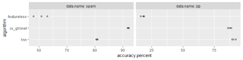
visualized using the figure below,
library(ggplot2)
ggplot()+
  geom_point(aes(
    accuracy.percent, algorithm),
    shape=1,
    data=accuracy.dt)+
  facet_grid(. ~ data.name, labeller=label_both, scales="free")

mlr3
There are a number of differences between the code we wrote above, and the code we write using the mlr3 framework.
- in mlr3 terms, we did benchmarking.
- in mlr3 we need to use Learners (instances of R6 class) rather than directly calling the learn/predict functions.
- man page for nearest neighbors classification.
- man page for regularized linear model.
- in mlr3 terms, each data set is represented as a Task, which can be created from a data table.
- reference about how to set hyper-params in mlr3 (in for loop code above we can set number of neighbors when calling knn function, and it defaulted to 1).
First we create a list of tasks, each one representing a data set:
list.of.tasks <- list()
for(data.name in names(data.list)){
  one.data <- data.list[[data.name]]
  one.dt <- with(one.data, data.table(input.mat, output.vec))
  list.of.tasks[[data.name]] <- mlr3::TaskClassif$new(
    data.name, one.dt, target="output.vec")
}
list.of.tasks
## $zip
## <TaskClassif:zip> (2007 x 257)
## * Target: output.vec
## * Properties: multiclass
## * Features (256):
##   - dbl (256): V10, V100, V101, V102, V103, V104, V105, V106, V107,
##     V108, V109, V11, V110, V111, V112, V113, V114, V115, V116, V117,
##     V118, V119, V12, V120, V121, V122, V123, V124, V125, V126, V127,
##     V128, V129, V13, V130, V131, V132, V133, V134, V135, V136, V137,
##     V138, V139, V14, V140, V141, V142, V143, V144, V145, V146, V147,
##     V148, V149, V15, V150, V151, V152, V153, V154, V155, V156, V157,
##     V158, V159, V16, V160, V161, V162, V163, V164, V165, V166, V167,
##     V168, V169, V17, V170, V171, V172, V173, V174, V175, V176, V177,
##     V178, V179, V18, V180, V181, V182, V183, V184, V185, V186, V187,
##     V188, V189, V19, [...]
##
## $spam
## <TaskClassif:spam> (4601 x 58)
## * Target: output.vec
## * Properties: twoclass
## * Features (57):
##   - dbl (57): V1, V10, V11, V12, V13, V14, V15, V16, V17, V18, V19, V2,
##     V20, V21, V22, V23, V24, V25, V26, V27, V28, V29, V3, V30, V31,
##     V32, V33, V34, V35, V36, V37, V38, V39, V4, V40, V41, V42, V43,
##     V44, V45, V46, V47, V48, V49, V5, V50, V51, V52, V53, V54, V55,
##     V56, V57, V6, V7, V8, V9
The code above defines the list of tasks / data sets.
The code below defines the learning algorithms. Note how we set hyper-parameters (k=1 neighbor, scale=FALSE) to obtain a consistent result with previous for loop code.
nn.learner <- mlr3learners::LearnerClassifKKNN$new()
nn.learner$param_set$values <- list(k=1, scale=FALSE)
nn.learner$id <- "classif.1nn"
(list.of.learners <- list(
  nn.learner,
  mlr3learners::LearnerClassifCVGlmnet$new(),
  mlr3::LearnerClassifFeatureless$new()))
## [[1]]
## <LearnerClassifKKNN:classif.1nn>: k-Nearest-Neighbor
## * Model: -
## * Parameters: k=1, scale=FALSE
## * Packages: mlr3, mlr3learners, kknn
## * Predict Types:  [response], prob
## * Feature Types: logical, integer, numeric, factor, ordered
## * Properties: multiclass, twoclass
##
## [[2]]
## <LearnerClassifCVGlmnet:classif.cv_glmnet>: GLM with Elastic Net Regularization
## * Model: -
## * Parameters: list()
## * Packages: mlr3, mlr3learners, glmnet
## * Predict Types:  [response], prob
## * Feature Types: logical, integer, numeric
## * Properties: multiclass, selected_features, twoclass, weights
##
## [[3]]
## <LearnerClassifFeatureless:classif.featureless>: Featureless Classification Learner
## * Model: -
## * Parameters: method=mode
## * Packages: mlr3
## * Predict Types:  [response], prob
## * Feature Types: logical, integer, numeric, character, factor, ordered,
##   POSIXct
## * Properties: featureless, importance, missings, multiclass,
##   selected_features, twoclass
Below we define the benchmark grid, (combinations of data sets and learning algorithms)
set.seed(1)
(benchmark.design <- mlr3::benchmark_grid(
  list.of.tasks,
  list.of.learners,
  mlr3::rsmp("cv", folds = n.folds)))
##    task             learner resampling
## 1:  zip         classif.1nn         cv
## 2:  zip   classif.cv_glmnet         cv
## 3:  zip classif.featureless         cv
## 4: spam         classif.1nn         cv
## 5: spam   classif.cv_glmnet         cv
## 6: spam classif.featureless         cv
Below we run the experiment,
benchmark.result <- mlr3::benchmark(benchmark.design)
## INFO  [14:44:07.045] [mlr3] Running benchmark with 18 resampling iterations
## INFO  [14:44:07.125] [mlr3] Applying learner 'classif.1nn' on task 'zip' (iter 1/3)
## INFO  [14:44:07.203] [mlr3] Applying learner 'classif.1nn' on task 'zip' (iter 2/3)
## INFO  [14:44:07.289] [mlr3] Applying learner 'classif.1nn' on task 'zip' (iter 3/3)
## INFO  [14:44:07.370] [mlr3] Applying learner 'classif.cv_glmnet' on task 'zip' (iter 1/3)
## INFO  [14:44:07.448] [mlr3] Applying learner 'classif.cv_glmnet' on task 'zip' (iter 2/3)
## INFO  [14:44:07.538] [mlr3] Applying learner 'classif.cv_glmnet' on task 'zip' (iter 3/3)
## INFO  [14:44:07.607] [mlr3] Applying learner 'classif.featureless' on task 'zip' (iter 1/3)
## INFO  [14:44:07.703] [mlr3] Applying learner 'classif.featureless' on task 'zip' (iter 2/3)
## INFO  [14:44:07.778] [mlr3] Applying learner 'classif.featureless' on task 'zip' (iter 3/3)
## INFO  [14:44:07.848] [mlr3] Applying learner 'classif.1nn' on task 'spam' (iter 1/3)
## INFO  [14:44:07.923] [mlr3] Applying learner 'classif.1nn' on task 'spam' (iter 2/3)
## INFO  [14:44:08.015] [mlr3] Applying learner 'classif.1nn' on task 'spam' (iter 3/3)
## INFO  [14:44:08.425] [mlr3] Applying learner 'classif.cv_glmnet' on task 'spam' (iter 1/3)
## INFO  [14:44:08.530] [mlr3] Applying learner 'classif.cv_glmnet' on task 'spam' (iter 2/3)
## INFO  [14:44:08.639] [mlr3] Applying learner 'classif.cv_glmnet' on task 'spam' (iter 3/3)
## INFO  [14:44:09.364] [mlr3] Applying learner 'classif.featureless' on task 'spam' (iter 1/3)
## INFO  [14:44:10.077] [mlr3] Applying learner 'classif.featureless' on task 'spam' (iter 2/3)
## INFO  [14:44:10.786] [mlr3] Applying learner 'classif.featureless' on task 'spam' (iter 3/3)
## INFO  [14:44:34.848] [mlr3] Finished benchmark
(score.dt <- benchmark.result$score())
##     nr task_id          learner_id resampling_id iteration classif.ce
##  1:  1     zip         classif.1nn            cv         1 0.10612855
##  2:  1     zip         classif.1nn            cv         2 0.07772795
##  3:  1     zip         classif.1nn            cv         3 0.09715994
##  4:  2     zip   classif.cv_glmnet            cv         1 0.14200299
##  5:  2     zip   classif.cv_glmnet            cv         2 0.11509716
##  6:  2     zip   classif.cv_glmnet            cv         3 0.12556054
##  7:  3     zip classif.featureless            cv         1 0.83707025
##  8:  3     zip classif.featureless            cv         2 0.81016442
##  9:  3     zip classif.featureless            cv         3 0.81614350
## 10:  4    spam         classif.1nn            cv         1 0.19035202
## 11:  4    spam         classif.1nn            cv         2 0.19361147
## 12:  4    spam         classif.1nn            cv         3 0.19439008
## 13:  5    spam   classif.cv_glmnet            cv         1 0.07822686
## 14:  5    spam   classif.cv_glmnet            cv         2 0.08148631
## 15:  5    spam   classif.cv_glmnet            cv         3 0.08284410
## 16:  6    spam classif.featureless            cv         1 0.39178618
## 17:  6    spam classif.featureless            cv         2 0.37092568
## 18:  6    spam classif.featureless            cv         3 0.41943901
## Hidden columns: uhash, task, learner, resampling, prediction
Above we see the output of the score function, which returns the evaluation metrics on the test set. Overall the code above is very well organized, and we only need a for loop over data sets (other for loops over the provided lists/rsmp folds happen inside of the benchmark function call). Below we convert column names for consistency with the previous section,
(mlr3.dt <- score.dt[, .(
  data.name=task_id,
  test.fold=iteration,
  algorithm=sub("classif.", "", learner_id),
  accuracy.percent = 100*(1-classif.ce)
)])
##     data.name test.fold   algorithm accuracy.percent
##  1:       zip         1         1nn         89.38714
##  2:       zip         2         1nn         92.22720
##  3:       zip         3         1nn         90.28401
##  4:       zip         1   cv_glmnet         85.79970
##  5:       zip         2   cv_glmnet         88.49028
##  6:       zip         3   cv_glmnet         87.44395
##  7:       zip         1 featureless         16.29297
##  8:       zip         2 featureless         18.98356
##  9:       zip         3 featureless         18.38565
## 10:      spam         1         1nn         80.96480
## 11:      spam         2         1nn         80.63885
## 12:      spam         3         1nn         80.56099
## 13:      spam         1   cv_glmnet         92.17731
## 14:      spam         2   cv_glmnet         91.85137
## 15:      spam         3   cv_glmnet         91.71559
## 16:      spam         1 featureless         60.82138
## 17:      spam         2 featureless         62.90743
## 18:      spam         3 featureless         58.05610
Below we plot the results,
ggplot()+
  geom_point(aes(
    accuracy.percent, algorithm),
    shape=1,
    data=mlr3.dt)+
  facet_grid(. ~ data.name, labeller=label_both, scales="free")
What if we wanted to tune the number of neighbors? (select the best value using cross-validation, rather than just using 1 neighbor which may overfit) Exercise for the reader: use mlr3tuning::auto_tuner to implement that as another learner in this section.
What if we wanted to compute AUC in addition to accuracy? mlr3
docs
explain that you can provide measures as an argument to the $score()
function. Exercise for the reader:
- set
learner$predict_type <- "prob"so that a real-valued score is output (rather than a class). - for binary you can use typical AUC, see mlr3 measure docs.
- for multiclass you can use an AUC generalization, see mlr3 measure docs.
- use
benchmark.result$score(list.of.measures)to compute a table of results.
What if you wanted to run the benchmark experiment in parallel?
Exercise for the reader: declare a future::plan("multisession") to
do that, see mlr3 benchmark
docs.
tidymodels
Tidymodels is newer framework with similar goals as mlr3, but it has some disadvantages.
- since it is newer, there is some functionality which is not yet implemented, such as running models on several data sets (equivalent of mlr3’s list of tasks in benchmark_grid). The closest analog would be workflowsets which allows one to specify a list of models/learners, but currently you have to use a for loop over data sets.
- the nomenclature on data splitting is unclear and potentially confusing (see discussion below).
https://www.tidymodels.org/start/case-study/#data-split explains has confusing/conflicting names for sets.
- The nomenclature I typically use is derived from the Deep Learning book. The full data set is split into train and test sets, then the train set is split into subtrain and validation sets. This nomenclature is great because it is unambiguous, unlike the tidymodels nomenclature which uses multiple names for the same set, and the same name for multiple different sets.
- the functions
initial_split,trainingandtestingare used, “let’s reserve 25% of the stays to the test set” - I believe this is my train/test split. - “we’ve relied on 10-fold cross-validation as the primary resampling method using rsample::vfold_cv(). This has created 10 different resamples of the training set (which we further split into analysis and assessment sets)” - I believe tidymodels “training” is my train set, split into “analysis” (my subtrain) and “assessment” (my validation).
- “let’s create a single resample called a validation set. In tidymodels, a validation set is treated as a single iteration of resampling. This will be a split from the 37,500 stays that were not used for testing, which we called hotel_other” - I believe tidymodels “other” is my train set.
- “This split creates two new datasets: the set held out for the purpose of measuring performance, called the validation set, and the remaining data used to fit the model, called the training set.” - I believe tidymodels “validation” is the same as mine, whereas tidymodels “training” is my subtrain.
- Overall the tidymodels nomenclature can be potentially confusing.
- my train set is called “other” or “training” in tidymodels.
- my subtrain set is called “analysis” or “training” in tidymodels.
- my validation set is called “assessment” or “validation” in tidymodels.
Chapter 11 of Tidy Modeling With R online book explains how to use workflowsets to compare models with resampling (testing). Getting started materials has an intro to resampling in tidymodels.
Models/algorithms
- null model is featureless baseline.
- nearest neighbors
- Regularized linear model
tidy.stats.dt.list <- list()
tidy.acc.dt.list <- list()
for(data.name in names(data.list)){
  one.data <- data.list[[data.name]]
  one.dt <- with(one.data, data.table(input.mat, output.vec))
  vfold.obj <- rsample::vfold_cv(one.dt, n.folds)
  my.workflow.set <- workflowsets::workflow_set(
    preproc = list(
      base=recipes::recipe(output.vec ~ ., data=one.dt)),
    models = list(
      featureless = parsnip::null_model(mode="classification") |>
        parsnip::set_engine("parsnip"),
      ## TODO: how to fix error? 2 of 3 resampling: base_cv_glmnet failed with: 1 argument has been tagged for tuning in this component: model_spec. Please use one of the tuning functions (e.g. `tune_grid()`) to optimize them.
      ## cv_glmnet = parsnip::multinom_reg(penalty = tune::tune(), mixture = 1) |>
      ##   parsnip::set_engine("glmnet"),
      "1nn" = parsnip::nearest_neighbor(mode="classification", neighbors=1)
    )
  ) |> workflowsets::workflow_map(
    "fit_resamples",
    ## Options to `workflow_map()`:
    seed = 1101, verbose = TRUE,
    ## Options to `fit_resamples()`:
    resamples = vfold.obj)
  tidy.stats.dt.list[[data.name]] <- data.table(
    data.name,
    workflowsets::collect_metrics(my.workflow.set)
  )[.metric=="accuracy"]
  for(algo.i in seq_along(my.workflow.set$result)){
    result.tib <- my.workflow.set$result[[algo.i]]
    tidy.acc.dt.list[[paste(data.name, algo.i)]] <- data.table::rbindlist(
      result.tib[[".metrics"]]
    )[.metric=="accuracy", .(
      data.name,
      test.fold=as.integer(sub("Fold", "", result.tib$id)),
      algorithm=sub("base_", "", my.workflow.set$wflow_id[algo.i]),
      accuracy.percent=.estimate*100
    )]
  }
}
## i 1 of 2 resampling: base_featureless
## ✔ 1 of 2 resampling: base_featureless (721ms)
## i 2 of 2 resampling: base_1nn
## ✔ 2 of 2 resampling: base_1nn (3.2s)
## i 1 of 2 resampling: base_featureless
## ✔ 1 of 2 resampling: base_featureless (200ms)
## i 2 of 2 resampling: base_1nn
## ✔ 2 of 2 resampling: base_1nn (2.8s)
(tidy.stats.dt <- rbindlist(tidy.stats.dt.list))
##    data.name         wflow_id              .config preproc            model
## 1:       zip base_featureless Preprocessor1_Model1  recipe       null_model
## 2:       zip         base_1nn Preprocessor1_Model1  recipe nearest_neighbor
## 3:      spam base_featureless Preprocessor1_Model1  recipe       null_model
## 4:      spam         base_1nn Preprocessor1_Model1  recipe nearest_neighbor
##     .metric .estimator      mean n      std_err
## 1: accuracy multiclass 0.1788739 3 0.0114923394
## 2: accuracy multiclass 0.8883906 3 0.0070287673
## 3: accuracy     binary 0.6059550 3 0.0008453037
## 4: accuracy     binary 0.9034998 3 0.0019782561
(tidy.acc.dt <- rbindlist(tidy.acc.dt.list))
##     data.name test.fold   algorithm accuracy.percent
##  1:       zip         1 featureless         15.69507
##  2:       zip         2 featureless         18.38565
##  3:       zip         3 featureless         19.58146
##  4:       zip         1         1nn         89.38714
##  5:       zip         2         1nn         87.44395
##  6:       zip         3         1nn         89.68610
##  7:      spam         1 featureless         60.75619
##  8:      spam         2 featureless         60.56063
##  9:      spam         3 featureless         60.46967
## 10:      spam         1         1nn         90.48240
## 11:      spam         2         1nn         89.96089
## 12:      spam         3         1nn         90.60665
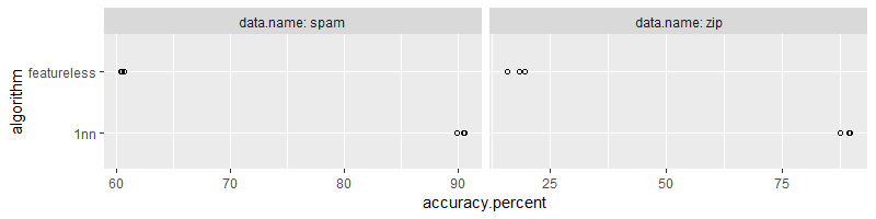
The code above computes nearest neighbors and featureless predictions,
and stores prediction accuracy for each test set in tidy.acc.dt
(which is rather complicated). It is a bit easier to compute
tidy.stats.dt which is the mean and SD of accuracy over test
folds. We visualize this data below,
ggplot()+
  geom_point(aes(
    accuracy.percent, algorithm),
    shape=1,
    data=tidy.acc.dt)+
  facet_grid(. ~ data.name, labeller=label_both, scales="free")
Comparison
Below we compute the combined data table,
(compare.dt <- rbind(
  data.table(package="base", accuracy.dt),
  data.table(package="tidymodels", tidy.acc.dt),
  data.table(package="mlr3", mlr3.dt)))
##        package data.name test.fold   algorithm accuracy.percent
##  1:       base       zip         1   cv_glmnet         85.65022
##  2:       base       zip         1 featureless         16.29297
##  3:       base       zip         1         1nn         89.38714
##  4:       base       zip         2   cv_glmnet         88.49028
##  5:       base       zip         2 featureless         18.98356
##  6:       base       zip         2         1nn         92.22720
##  7:       base       zip         3   cv_glmnet         87.14499
##  8:       base       zip         3 featureless         18.38565
##  9:       base       zip         3         1nn         90.28401
## 10:       base      spam         1   cv_glmnet         91.85137
## 11:       base      spam         1 featureless         60.82138
## 12:       base      spam         1         1nn         79.85658
## 13:       base      spam         2   cv_glmnet         92.56845
## 14:       base      spam         2 featureless         61.66884
## 15:       base      spam         2         1nn         81.29074
## 16:       base      spam         3   cv_glmnet         91.06327
## 17:       base      spam         3 featureless         59.29550
## 18:       base      spam         3         1nn         82.51794
## 19: tidymodels       zip         1 featureless         15.69507
## 20: tidymodels       zip         2 featureless         18.38565
## 21: tidymodels       zip         3 featureless         19.58146
## 22: tidymodels       zip         1         1nn         89.38714
## 23: tidymodels       zip         2         1nn         87.44395
## 24: tidymodels       zip         3         1nn         89.68610
## 25: tidymodels      spam         1 featureless         60.75619
## 26: tidymodels      spam         2 featureless         60.56063
## 27: tidymodels      spam         3 featureless         60.46967
## 28: tidymodels      spam         1         1nn         90.48240
## 29: tidymodels      spam         2         1nn         89.96089
## 30: tidymodels      spam         3         1nn         90.60665
## 31:       mlr3       zip         1         1nn         89.38714
## 32:       mlr3       zip         2         1nn         92.22720
## 33:       mlr3       zip         3         1nn         90.28401
## 34:       mlr3       zip         1   cv_glmnet         85.79970
## 35:       mlr3       zip         2   cv_glmnet         88.49028
## 36:       mlr3       zip         3   cv_glmnet         87.44395
## 37:       mlr3       zip         1 featureless         16.29297
## 38:       mlr3       zip         2 featureless         18.98356
## 39:       mlr3       zip         3 featureless         18.38565
## 40:       mlr3      spam         1         1nn         80.96480
## 41:       mlr3      spam         2         1nn         80.63885
## 42:       mlr3      spam         3         1nn         80.56099
## 43:       mlr3      spam         1   cv_glmnet         92.17731
## 44:       mlr3      spam         2   cv_glmnet         91.85137
## 45:       mlr3      spam         3   cv_glmnet         91.71559
## 46:       mlr3      spam         1 featureless         60.82138
## 47:       mlr3      spam         2 featureless         62.90743
## 48:       mlr3      spam         3 featureless         58.05610
##        package data.name test.fold   algorithm accuracy.percent
Below we plot the numbers from different frameworks together for comparison,
ggplot()+
  geom_point(aes(
    accuracy.percent, package),
    shape=1,
    data=compare.dt)+
  facet_grid(algorithm ~ data.name, labeller=label_both, scales="free")
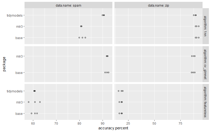
In the plot above we see that the nearest neighbors algorithm is more accuracy in tidymodels, which is because I could not figure out a way to turn off scaling. Exercise for the reader: modify the for loop and mlr3 code to do scaling, so that the nearest neighbors algorithm is as accurate as in tidymodels.
Conclusions
We have explored how to code cross-validation using three methods: base R for loop, mlr3 package, tidymodels package. We have seen that mlr3 gives consistent results with the base R for loop, whereas tidymodels has some limitations (no easy way to implement auto tuning glmnet, no consistent names for split sets, not easy to compute test accuracy for each fold, etc). Overall I would recommend using base R for loops for full control, or mlr3 if you are doing standard cross-validation experiments like the one we explored above.
Related work
Louis Aslett wrote lecture notes for tidymodels and mlr3.
version info
sessionInfo()
## R version 4.3.2 (2023-10-31 ucrt)
## Platform: x86_64-w64-mingw32/x64 (64-bit)
## Running under: Windows 10 x64 (build 19045)
##
## Matrix products: default
##
##
## locale:
## [1] LC_COLLATE=English_United States.utf8
## [2] LC_CTYPE=English_United States.utf8
## [3] LC_MONETARY=English_United States.utf8
## [4] LC_NUMERIC=C
## [5] LC_TIME=English_United States.utf8
##
## time zone: America/Phoenix
## tzcode source: internal
##
## attached base packages:
## [1] stats     graphics  grDevices utils     datasets  methods   base
##
## other attached packages:
## [1] kknn_1.3.1        parsnip_1.1.1     recipes_1.0.8     dplyr_1.1.4
## [5] ggplot2_3.4.4     data.table_1.14.8
##
## loaded via a namespace (and not attached):
##  [1] tidyselect_1.2.0     timeDate_4022.108    farver_2.1.1
##  [4] R.utils_2.12.3       paradox_0.11.1       digest_0.6.33
##  [7] rpart_4.1.21         timechange_0.2.0     lifecycle_1.0.4
## [10] ellipsis_0.3.2       yardstick_1.2.0      survival_3.5-7
## [13] magrittr_2.0.3       compiler_4.3.2       rlang_1.1.2
## [16] tools_4.3.2          igraph_1.5.1         utf8_1.2.4
## [19] knitr_1.45           prettyunits_1.2.0    labeling_0.4.3
## [22] DiceDesign_1.9       withr_2.5.2          purrr_1.0.2
## [25] mlr3misc_0.13.0      workflows_1.1.3      R.oo_1.25.0
## [28] nnet_7.3-19          grid_4.3.2           tune_1.1.2
## [31] fansi_1.0.5          mlr3measures_0.5.0   colorspace_2.1-0
## [34] future_1.33.0        globals_0.16.2       scales_1.3.0
## [37] iterators_1.0.14     MASS_7.3-60          cli_3.6.1
## [40] crayon_1.5.2         generics_0.1.3       future.apply_1.11.0
## [43] splines_4.3.2        dials_1.2.0          parallel_4.3.2
## [46] vctrs_0.6.4          hardhat_1.3.0        glmnet_4.1-8
## [49] Matrix_1.6-3         listenv_0.9.0        mlr3learners_0.5.7
## [52] foreach_1.5.2        lgr_0.4.4            gower_1.0.1
## [55] tidyr_1.3.0          glue_1.6.2           parallelly_1.36.0
## [58] codetools_0.2-19     rsample_1.2.0        lubridate_1.9.3
## [61] shape_1.4.6          gtable_0.3.4         mlr3_0.17.0
## [64] palmerpenguins_0.1.1 munsell_0.5.0        GPfit_1.0-8
## [67] tibble_3.2.1         furrr_0.3.1          pillar_1.9.0
## [70] workflowsets_1.0.1   ipred_0.9-14         lava_1.7.3
## [73] R6_2.5.1             lhs_1.1.6            evaluate_0.23
## [76] lattice_0.22-5       highr_0.10           R.methodsS3_1.8.2
## [79] backports_1.4.1      class_7.3-22         Rcpp_1.0.11
## [82] uuid_1.1-1           prodlim_2023.08.28   checkmate_2.3.0
## [85] xfun_0.41            pkgconfig_2.0.3