Historical reverse imports
I recently read Norm Matloff’s TidyverseSkeptic essay, which describes the advantages of teaching base R, in contrast to teaching using the tidyverse (which is a collection of R packages which re-implements some base R functionality using a different API). I think that two properties of the tidyverse make it difficult to use and teach, (1) there are so many different packages and functions, and (2) the packages are changed (and functions deprecated) so frequently. You could make an argument that base R also suffers from (1) – there are a lot of functions in base R. But base R has a clear win in (2), due to its focus on backwards compatibility.
Another package which re-implements some base R functionality is data.table, which provides some functions for reading/writing CSV files (fread/fwrite), reshaping data (melt/dcast), and aggregation by group (single square bracket with by argument). Base R has similar functions for each purpose (read.csv, write.csv, reshape, tapply). Similar tidyverse functions are provided in three different packages (readr, tidyr, dplyr). There is an older/deprecated version of data reshaping in the reshape2 package, and an older/deprecated version of aggregation by group in the plyr package. I studied some of these functions in my recent R Journal research paper on data reshaping.
I use data.table for research and teaching, and I find that it is quite easy to use for both purposes, because of its terse SQL-like syntax, and the relatively small number of functions and concepts that need to be learned. Its efficiency is a major reason that I keep using R for most of my research. Norm Matloff described data.table as “a technically superior competitor to dplyr.” So I would expect that there would be a large number of people using data.table. But Norm Matloff claims that there are even more people using tidyverse due to RStudio’s marketing. To what extent is that true?
We can tell how many other R package developers are using a given R package by looking at the reverse dependencies on the corresponding CRAN pages. For example the CRAN page for data.table currently lists about a full web browser screen full of other packages under Reverse imports, meaning other packages which Import and use at least one function from data.table. That seems like a lot, but is it? I looked at the corresponding page for dplyr and it was at least twice as large. Has that always been the case? Did data.table ever have more reverse dependencies than dplyr? I set about to quickly answer these questions using the R code below.
The reverse dependencies for each CRAN package are stored in the packages.rds file (currently a 7.3MB binary file that can be read into R using the readRDS function). But that file just has the most recent data. What about historical data?
Lucky for us, the Microsoft R Application Network (MRAN) keeps a time machine of daily CRAN snapshots, so we can access historical packages.rds files going back to its inception on September 17th, 2014. For example here is how we would download the data from that first day:
library(data.table)
get_packages <- function(date){
  date.str <- paste(date)
  date.dir <- file.path("~/R/dt-deps-time", date.str)
  dir.create(date.dir,showWarnings=FALSE,recursive=TRUE)
  packages.rds <- file.path(date.dir, "packages.rds")
  if(!file.exists(packages.rds)){
    u <- paste0(
      "https://cran.microsoft.com/snapshot/",
      date.str,
      "/web/packages/packages.rds")
    print(packages.rds)
    download.file(u, packages.rds)
  }
  packages <- readRDS(packages.rds)
  data.table(packages)
}
pkg.dt <- get_packages("2014-09-17")
names(pkg.dt)
##  [1] "Package"                 "Version"
##  [3] "Priority"                "Depends"
##  [5] "Imports"                 "LinkingTo"
##  [7] "Suggests"                "Enhances"
##  [9] "License"                 "License_is_FOSS"
## [11] "License_restricts_use"   "OS_type"
## [13] "Archs"                   "MD5sum"
## [15] "NeedsCompilation"        "Authors@R"
## [17] "Author"                  "BugReports"
## [19] "Contact"                 "Copyright"
## [21] "Description"             "Encoding"
## [23] "Language"                "Maintainer"
## [25] "Title"                   "URL"
## [27] "SystemRequirements"      "Type"
## [29] "Path"                    "Classification/ACM"
## [31] "Classification/JEL"      "Classification/MSC"
## [33] "Published"               "VignetteBuilder"
## [35] "Additional_repositories" "Reverse depends"
## [37] "Reverse imports"         "Reverse linking to"
## [39] "Reverse suggests"        "Reverse enhances"
## [41] "MD5sum"
(rev.imports.str <- pkg.dt["data.table", on="Package"][["Reverse imports"]])
## [1] "aLFQ, benford.analysis, Causata, DataCombine, eeptools, FAOSTAT, freqweights, gems, IAT, Kmisc, lar, lllcrc, miscset, optiRum, pxweb, qdapTools, randomNames, RAPIDR, RbioRXN, rbison, rfisheries, rgauges, rgbif, rlist, rnoaa, rplos, SGP, simPH, spocc, sweSCB, taxize, treebase, treemap"
We can see from the output above that the Reverse imports are stored as a text string, each package separated by a comma and space. We can get the reverse imports via a regular expression,
nc::capture_all_str(rev.imports.str, dep.pkg="[^, ]+")
##              dep.pkg
##               <char>
##  1:             aLFQ
##  2: benford.analysis
##  3:          Causata
##  4:      DataCombine
##  5:         eeptools
##  6:          FAOSTAT
##  7:      freqweights
##  8:             gems
##  9:              IAT
## 10:            Kmisc
## 11:              lar
## 12:           lllcrc
## 13:          miscset
## 14:          optiRum
## 15:            pxweb
## 16:        qdapTools
## 17:      randomNames
## 18:           RAPIDR
## 19:          RbioRXN
## 20:           rbison
## 21:       rfisheries
## 22:          rgauges
## 23:            rgbif
## 24:            rlist
## 25:            rnoaa
## 26:            rplos
## 27:              SGP
## 28:            simPH
## 29:            spocc
## 30:           sweSCB
## 31:           taxize
## 32:         treebase
## 33:          treemap
##              dep.pkg
or by splitting on the delimiter,
strsplit(rev.imports.str, ", ")[[1]]
##  [1] "aLFQ"             "benford.analysis" "Causata"          "DataCombine"
##  [5] "eeptools"         "FAOSTAT"          "freqweights"      "gems"
##  [9] "IAT"              "Kmisc"            "lar"              "lllcrc"
## [13] "miscset"          "optiRum"          "pxweb"            "qdapTools"
## [17] "randomNames"      "RAPIDR"           "RbioRXN"          "rbison"
## [21] "rfisheries"       "rgauges"          "rgbif"            "rlist"
## [25] "rnoaa"            "rplos"            "SGP"              "simPH"
## [29] "spocc"            "sweSCB"           "taxize"           "treebase"
## [33] "treemap"
Here is a function for returning the number of reverse imports for selected packages, for a given packages table:
get_num_rev_imports <- function(packages.dt, some.pkg.names){
  packages.dt[some.pkg.names, .(
    Package,
    n.rev.imports=sapply(strsplit(`Reverse imports`, ", "), length)
  ), on="Package"]
}
compare.pkgs <- c("data.table","dplyr","plyr","tidyr","readr","reshape2")
get_num_rev_imports(pkg.dt, compare.pkgs)
##       Package n.rev.imports
##        <char>         <int>
## 1: data.table            33
## 2:      dplyr            11
## 3:       plyr           167
## 4:      tidyr             1
## 5:      readr             1
## 6:   reshape2            87
Let’s look at the first day of every month since the start of 2015.
date.vec <- seq(as.IDate("2015-01-01"), as.IDate("2022-01-01"), by="month")
(rev.imp.counts <- data.table(date=date.vec)[, {
  date.pkgs <- get_packages(date)
  get_num_rev_imports(date.pkgs, compare.pkgs)
}, by=date])
##            date    Package n.rev.imports
##          <IDat>     <char>         <int>
##   1: 2015-01-01 data.table            39
##   2: 2015-01-01      dplyr            27
##   3: 2015-01-01       plyr           198
##   4: 2015-01-01      tidyr             2
##   5: 2015-01-01      readr             1
##  ---
## 506: 2022-01-01      dplyr          2750
## 507: 2022-01-01       plyr           822
## 508: 2022-01-01      tidyr          1296
## 509: 2022-01-01      readr           473
## 510: 2022-01-01   reshape2           745
Finally we can plug these count data into a ggplot,
library(ggplot2)
expand.days <- 11*30
gg <- ggplot()+
  theme_bw()+
  scale_color_manual(values=c(
    plyr="grey50",
    reshape2="grey50",
    data.table="blue",
    tidyr="red",
    readr="red",
    dplyr="red"))+
  scale_x_date(
    breaks=seq(min(date.vec), max(date.vec), by="year"),
    limits=as.IDate(c(
      min(date.vec)-expand.days,
      max(date.vec)+expand.days
    )))
gg.imports <- gg+
  scale_y_log10()+
  geom_line(aes(
    date, n.rev.imports, color=Package),
    size=1,
    data=rev.imp.counts)
directlabels::direct.label(
  gg.imports,
  directlabels::dl.combine("left.polygons", "right.polygons"))
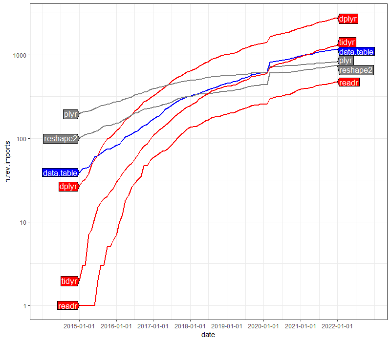
We can see in the figure above that at the beginning of this time period, data.table had more reverse imports than readr/dplyr/tidyr (red), but fewer than plyr/reshape2 (grey). At the end of this time period we see the opposite pattern, which makes sense because plyr/reshape2 are now deprecated (it is actually surprising to see their reverse imports increasing over time). The number of reverse imports of dplyr surpassed that of data.table in 2015, and the same happened for tidyr in 2021.
What about the rate of change each month? Overall each is clearly increasing, but which is increasing the most?
(rev.imp.diff <- rev.imp.counts[, .(
  diff.rev.imports=diff(n.rev.imports),
  date=date[-1]
), by=Package])
##         Package diff.rev.imports       date
##          <char>            <int>     <IDat>
##   1: data.table                4 2015-02-01
##   2: data.table                1 2015-03-01
##   3: data.table                1 2015-04-01
##   4: data.table                6 2015-05-01
##   5: data.table                9 2015-06-01
##  ---
## 500:   reshape2                7 2021-09-01
## 501:   reshape2               12 2021-10-01
## 502:   reshape2               12 2021-11-01
## 503:   reshape2                9 2021-12-01
## 504:   reshape2                4 2022-01-01
gg.diff <- gg+
  geom_line(aes(
    date, diff.rev.imports, color=Package),
    size=1,
    data=rev.imp.diff)+
  scale_y_continuous(
    "Monthly change in number of reverse imports",
    breaks=seq(0, 300, by=20))+
  coord_cartesian(ylim=c(-5, 100))
directlabels::direct.label(gg.diff, "right.polygons")
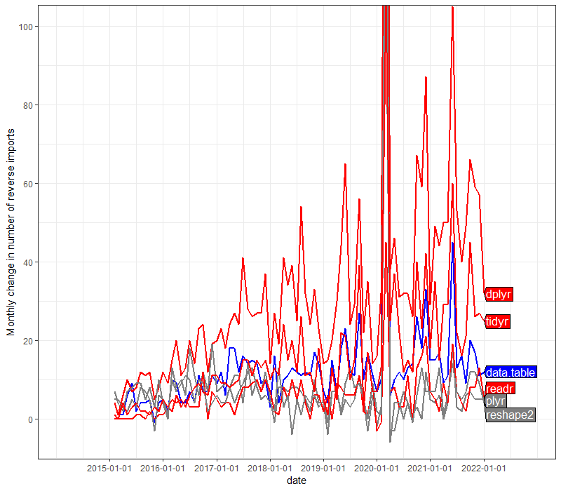
The figure above shows that the number of new reverse imports per month is around 10–100, with some variation over packages and over time.
Overall this analysis shows a few interesting trends.
- All packages, even ones that were deprecated, tend to have increased numbers of reverse imports over time.
- Tidyverse packages did not have as many reverse imports as data.table in 2015, but that trend has reversed in recent years.
Exercise for the reader: modify the code above to perform the same analysis for package properties other than Reverse imports (for example, Reverse depends and Reverse suggests). Plot each time series in a different panel/facet of a ggplot. Hint: use .SDcols with sapply as below!
some.cols <- c("Reverse imports", "Reverse depends", "Reverse suggests")
pkg.dt[compare.pkgs, .(
  dep.type=some.cols,
  n.rev.deps=sapply(.SD, function(x)length(strsplit(x, ", ")[[1]]))
), .SDcols=some.cols, by=.EACHI, on="Package"]
##        Package         dep.type n.rev.deps
##         <char>           <char>      <int>
##  1: data.table  Reverse imports         33
##  2: data.table  Reverse depends         13
##  3: data.table Reverse suggests          6
##  4:      dplyr  Reverse imports         11
##  5:      dplyr  Reverse depends          3
##  6:      dplyr Reverse suggests          5
##  7:       plyr  Reverse imports        167
##  8:       plyr  Reverse depends         50
##  9:       plyr Reverse suggests         40
## 10:      tidyr  Reverse imports          1
## 11:      tidyr  Reverse depends          1
## 12:      tidyr Reverse suggests          1
## 13:      readr  Reverse imports          1
## 14:      readr  Reverse depends          1
## 15:      readr Reverse suggests          1
## 16:   reshape2  Reverse imports         87
## 17:   reshape2  Reverse depends         20
## 18:   reshape2 Reverse suggests         26