Indirect reverse dependencies
For a recent grant proposal submission to the National Science
Foundation POSE program, I wanted to make an argument that the
data.table R package is one of the most used, out of all R
packages.
I therefore wrote some code to compute the number of indirect reverse dependencies for all R packages. First, download meta-data from the current CRAN,
library(data.table)
if(!file.exists("packages.rds")){
  u <- paste0(
    "https://cloud.r-project.org/web/packages/packages.rds")
  download.file(u, "packages.rds")
}
packages <- readRDS("packages.rds")
pkg.dt <- data.table(packages)[is.na(Path)]
nrow(pkg.dt)
## [1] 18761
The output above shows the number of packages on CRAN.
Direct reverse imports
Then, we can get direct reverse imports,
imp.by <- pkg.dt[, .(
  imported.by=strsplit(`Reverse imports`, ", ")[[1]]
), by=.(Imports=Package)]
imp.by[!is.na(imported.by)]
##            Imports imported.by
##             <char>      <char>
##     1:         abc  ecolottery
##     2:         abc       poems
##     3: ABCanalysis    EDOtrans
##     4:       abind    agroclim
##     5:       abind     alleHap
##    ---
## 79416:      ztable     rrtable
## 79417:      ztable        webr
## 79418:         zyp      fasstr
## 79419:         zyp  FlowScreen
## 79420:         zyp       gimms
The table above contains one row for each direct reverse import listed on CRAN.
imp.by[Imports=="data.table"]
##          Imports    imported.by
##           <char>         <char>
##    1: data.table  accessibility
##    2: data.table          actel
##    3: data.table ActivePathways
##    4: data.table  ActivityIndex
##    5: data.table        ADAMgui
##   ---
## 1323: data.table           yaps
## 1324: data.table  youngSwimmers
## 1325: data.table           zebu
## 1326: data.table       zeitgebr
## 1327: data.table zoomGroupStats
The table above contains a row for each direct reverse import listed
for the data.table package.
Indirect reverse imports
Then, we can use a loop to recursively compute indirect reverse imports,
order.i <- 0
ord.dt.list <- list()
order.pkgs <- pkg.dt[, .(Package, Imports=Package)]
while(nrow(order.pkgs)){
  print(order.i <- order.i+1)
  order.deps <- imp.by[
    order.pkgs,
    on="Imports", nomatch=0L, allow.cartesian=TRUE]
  if(nrow(order.deps)){
    ord.dt.list[[order.i]] <- data.table(order.i, order.deps)
  }
  order.pkgs <- unique(order.deps[, .(Package, Imports=imported.by)])
}
## [1] 1
## [1] 2
## [1] 3
## [1] 4
## [1] 5
## [1] 6
## [1] 7
## [1] 8
## [1] 9
## [1] 10
## [1] 11
## [1] 12
## [1] 13
## [1] 14
## [1] 15
## [1] 16
## [1] 17
(ord.dt <- do.call(rbind, ord.dt.list))
##          order.i     Imports imported.by    Package
##            <num>      <char>      <char>     <char>
##       1:       1          A3        <NA>         A3
##       2:       1    AATtools        <NA>   AATtools
##       3:       1      ABACUS        <NA>     ABACUS
##       4:       1  abbreviate        <NA> abbreviate
##       5:       1      abbyyR        <NA>     abbyyR
##      ---
## 2107718:      15       immcp        <NA>      rlang
## 2107719:      15 nlmixr2plot     nlmixr2      rlang
## 2107720:      16     nlmixr2        <NA>        cli
## 2107721:      16     nlmixr2        <NA>       glue
## 2107722:      16     nlmixr2        <NA>      rlang
The table above contains one row for each reverse import (direct or
indirect). Direct reverse imports have order.i=1 and indirect have
larger values.
Below we check that the number of packages in this table is the same as the number of packages in the CRAN meta-data,
rbind(pkgs.in.ord=length(unique(ord.dt$Package)), pkgs=nrow(pkg.dt))
##              [,1]
## pkgs.in.ord 18761
## pkgs        18761
The output above indicates that the table of reverse imports was computed correctly (the total number of packages is correct).
Subset of packages funded by NSF
Which packages were funded by NSF?
pkg.dt[, Desc.no.newlines := gsub("\n\\s+", " ", Description)]
(nsf.pkgs <- pkg.dt[
  grep("NSF|National Science Foundation", Desc.no.newlines),
  Package])
##  [1] "adaptivetau"         "BAS"                 "bizicount"
##  [4] "fastCorrDiff"        "fdapace"             "fields"
##  [7] "futureheatwaves"     "hurricaneexposure"   "hwep"
## [10] "LatticeKrig"         "melt"                "merDeriv"
## [13] "metagear"            "mined"               "mixtools"
## [16] "mosaic"              "mosaicData"          "MultNonParam"
## [19] "nonnest2"            "PHInfiniteEstimates" "PST"
## [22] "RealVAMS"            "rEMM"                "rmonad"
## [25] "SPlit"               "SPREDA"              "stream"
## [28] "supercompress"       "TAG"                 "telefit"
## [31] "tensr"
Which of the reverse imports were funded by NSF?
dt.pkgs <- ord.dt[Package=="data.table", imported.by]
(int.pkgs <- intersect(nsf.pkgs, dt.pkgs))
## [1] "bizicount"         "fdapace"           "futureheatwaves"
## [4] "hurricaneexposure"
The output above shows that there are four reverse imports that were also funded by NSF.
Computing path from reverse import in dependency graph
What is the path of packages from each reverse import in the dependency graph?
select.dt <- data.table(
  rev.dep=int.pkgs,
  imported.by=int.pkgs,
  Package="data.table")
path.dt.list <- list()
iteration <- 0
while(nrow(select.dt)){
  print(iteration <- iteration+1)
  dep.dt <- ord.dt[select.dt, on=.(imported.by, Package)]
  path.dt.list[[iteration]] <- dep.dt
  select.dt <- dep.dt[
    Imports != Package,
    .(rev.dep, imported.by=Imports, Package)]
}
## [1] 1
## [1] 2
## [1] 3
## [1] 4
(path.dt <- do.call(rbind, path.dt.list)[
  order(Package, rev.dep, -order.i),
  .(Package, rev.dep, order.i, imported.by, Imports)])
##       Package           rev.dep order.i       imported.by    Imports
##        <char>            <char>   <num>            <char>     <char>
## 1: data.table         bizicount       4         bizicount     DHARMa
## 2: data.table         bizicount       3            DHARMa        gap
## 3: data.table         bizicount       2               gap     plotly
## 4: data.table         bizicount       1            plotly data.table
## 5: data.table           fdapace       2           fdapace      Hmisc
## 6: data.table           fdapace       1             Hmisc data.table
## 7: data.table   futureheatwaves       1   futureheatwaves data.table
## 8: data.table hurricaneexposure       1 hurricaneexposure data.table
The table above shows that there are two direct reverse imports
(futureheatwaves, hurricaneexposure) for which the path length (max
order.i) is 1. The fdapace package imports Hmisc which imports
data.table (path length 2), whereas bizicount imports DHARMa
which imports gap which imports plotly which imports data.table
(path length 4).
Unique reverse imports, direct or all
The code below counts the number of unique reverse imports (either direct or all), for each CRAN package,
(dep.type.counts <- rbind(
  data.table(dep.type="all", max.order=Inf),
  data.table(dep.type="direct", max.order=1)
)[, {
  ord.dt[order.i <= max.order, .(
    rev.imports=length(unique(na.omit(imported.by)))
  ), by=Package
  ][, `:=`(
    rank=rank(-rev.imports),
    prop.bigger=1-rank(rev.imports)/.N
  )][order(rank)]
}, by=dep.type])
##        dep.type  Package rev.imports    rank  prop.bigger
##          <char>   <char>       <int>   <num>        <num>
##     1:      all magrittr        8638     1.0 0.000000e+00
##     2:      all    rlang        8469     2.0 5.330206e-05
##     3:      all     Rcpp        8413     3.0 1.066041e-04
##     4:      all     glue        8275     4.0 1.599062e-04
##     5:      all       R6        8011     5.0 2.132083e-04
##    ---
## 37518:   direct    ztpln           0 11616.5 6.191301e-01
## 37519:   direct    zTree           0 11616.5 6.191301e-01
## 37520:   direct    ztype           0 11616.5 6.191301e-01
## 37521:   direct     ZVCV           0 11616.5 6.191301e-01
## 37522:   direct   zzlite           0 11616.5 6.191301e-01
The data.table package appears near the top in terms of number of
dependent packages,
(dt.counts <- dep.type.counts[Package=="data.table"])
##    dep.type    Package rev.imports  rank  prop.bigger
##      <char>     <char>       <int> <num>        <num>
## 1:      all data.table        2663    45 0.0023452908
## 2:   direct data.table        1327    11 0.0005330206
The table above shows that data.table has
- 1326 direct reverse imports, which is rank 11 among CRAN packages (only 10 other packages, 0.05% of all CRAN packages, have a larger number of reverse imports).
- 2661 packages which import either directly or indirectly, which is rank 45 among CRAN packages (only 44 other packages, 0.2% of all CRAN packages, have a larger number).
Comparison with other CRAN packages
The code below can be used to compute a histogram of reverse import
counts, among all CRAN packages. To compute a histogram using a
data.table rolling join, we first need to look at the range of the
data, and then use the min/max to define the sequence of midpoints of
histogram bins.
log10(range(dep.type.counts$rev.imports))
## [1] -Inf 3.936413
log10.min <- 0
log10.max <- 4
(bin.dt <- data.table(
  log10.bin=c(-Inf,seq(log10.min, log10.max, by=0.5))
)[, bin := 10^log10.bin][, Bin := round(bin)][])
##     log10.bin          bin   Bin
##         <num>        <num> <num>
##  1:      -Inf     0.000000     0
##  2:       0.0     1.000000     1
##  3:       0.5     3.162278     3
##  4:       1.0    10.000000    10
##  5:       1.5    31.622777    32
##  6:       2.0   100.000000   100
##  7:       2.5   316.227766   316
##  8:       3.0  1000.000000  1000
##  9:       3.5  3162.277660  3162
## 10:       4.0 10000.000000 10000
The bins defined above range from 1 to 10000 on the log scale, with an additional bin for 0 (packages that have no reverse imports). Below we use a rolling join to figure out which packages are closest to each bin midpoint on the log scale,
dep.type.counts[, log10.rev.imports := log10(rev.imports)]
(bin.log.join <- bin.dt[dep.type.counts, .(
  dep.type, Package, Bin, bin,
  log10.bin=x.log10.bin,
  log10.rev.imports),
  roll="nearest",
  on=.(log10.bin=log10.rev.imports)])
##        dep.type  Package   Bin   bin log10.bin log10.rev.imports
##          <char>   <char> <num> <num>     <num>             <num>
##     1:      all magrittr 10000 10000         4          3.936413
##     2:      all    rlang 10000 10000         4          3.927832
##     3:      all     Rcpp 10000 10000         4          3.924951
##     4:      all     glue 10000 10000         4          3.917768
##     5:      all       R6 10000 10000         4          3.903687
##    ---
## 37518:   direct    ztpln     0     0      -Inf              -Inf
## 37519:   direct    zTree     0     0      -Inf              -Inf
## 37520:   direct    ztype     0     0      -Inf              -Inf
## 37521:   direct     ZVCV     0     0      -Inf              -Inf
## 37522:   direct   zzlite     0     0      -Inf              -Inf
The table above has columns for bin midpoint on the log scale,
log10.bin, as well as the actual number of reverse imports,
log10.rev.imports. We can compute a histogram by summarizing for
each bin,
(bin.log.hist <- bin.log.join[, .(
  n.packages=.N
), by=.(dep.type, bin)])
##     dep.type          bin n.packages
##       <char>        <num>      <int>
##  1:      all 10000.000000         18
##  2:      all  3162.277660         45
##  3:      all  1000.000000         68
##  4:      all   316.227766        111
##  5:      all   100.000000        211
##  6:      all    31.622777        379
##  7:      all    10.000000        673
##  8:      all     3.162278       1394
##  9:      all     1.000000       1572
## 10:      all     0.000000      14290
## 11:   direct  3162.277660          5
## 12:   direct  1000.000000         16
## 13:   direct   316.227766         58
## 14:   direct   100.000000        117
## 15:   direct    31.622777        276
## 16:   direct    10.000000        642
## 17:   direct     3.162278       1481
## 18:   direct     1.000000       1876
## 19:   direct     0.000000      14290
The table above has a column n.packages which shows the number of
packages which are closest to each bin. These numbers can be plotted
to compare with the corresponding number of reverse imports for the
data.table package,
library(ggplot2)
ggplot()+
  theme_bw()+
  geom_line(aes(
    bin, n.packages),
    color="grey50",
    size=2,
    data=bin.log.hist)+
  geom_vline(aes(
    xintercept=rev.imports),
    data=dt.counts)+
  geom_text(aes(
    rev.imports*0.9, Inf,
    label=sprintf(paste(
      "data.table rev. imports=%d",
      "rank=%d/%d packages",
      "%.2f%% of packages have",
      "larger rev. dep. count",
      sep="\n"),
      rev.imports, rank, nrow(pkg.dt), prop.bigger*100)),
    data=dt.counts,
    hjust=1,
    vjust=1.1)+
  facet_grid(. ~ dep.type, labeller=label_both)+
  scale_y_log10(paste(
    "Number of packages with that",
    "reverse dependency count (log scale)",
    sep="\n"))+
  scale_x_log10(paste(
    "Reverse dependency count",
    "(number of other packages which import, log scale)"))
## Warning: Transformation introduced infinite values in continuous x-
## axis
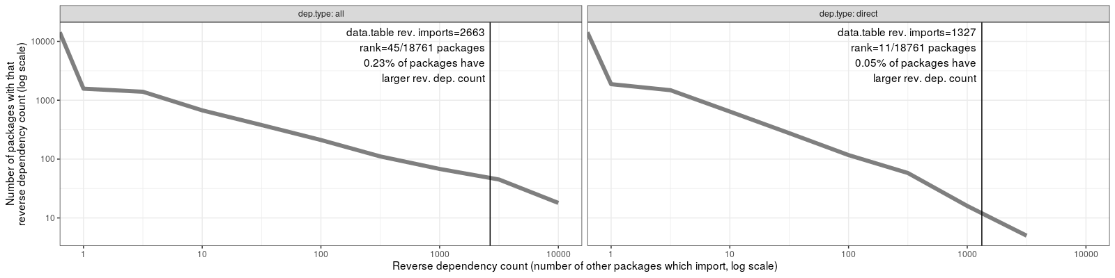
The figure above shows that data.table is ranked near the top, when
comparing with other CRAN packages in terms of number of reverse
imports.
Appendix: rolling join in original or log space?
In the code above, to compute a histogram that we want to display in the log space, we did a rolling join in the log space, which results in symmetric histogram bins. If we did the join in the original space, then the histogram bins would have been asymmetric, as the code below shows,
bin.tall <- melt(
  bin.dt[bin>0],
  measure.vars=c("log10.bin", "bin"),
  id.vars=c("Bin", "log10.bin"))
bin.tall[, next.break := c(value+c(diff(value)/2,NA)), by=variable]
bin.tall[, next.log10 := ifelse(
  variable=="bin", log10(next.break), next.break)]
bin.tall[, prev.log10 := c(NA, next.log10[-.N]), by=variable]
bin.tall[, distance := ifelse(variable=="bin", "original", "log")]
bin.not.na <- bin.tall[!(is.na(prev.log10)|is.na(next.log10))]
ggplot()+
  geom_segment(aes(
    prev.log10, distance,
    xend=next.log10, yend=distance),
    data=bin.not.na)+
  geom_point(aes(
    log10.bin, distance),
    data=bin.not.na)+
  facet_grid(. ~ Bin, labeller=label_both, scales="free")+
  scale_x_continuous(breaks=seq(log10.min, log10.max, by=0.1))

The figure above shows the center of each histogram bin as a dot, and the min/max extent of each bin as a line segment. It is clear that using original space distances for the join results in bins which are asymmetric, in the sense that the bin will count more data which is larger than the bin center.
Another way of looking at it is empirically, in terms of the reverse imports data,
bin.log.join[, log10.diff := ifelse(
  log10.rev.imports == -Inf, 0, log10.rev.imports-log10.bin)]
bin.width <- 0.05
ggplot()+
  geom_histogram(aes(
    log10.diff, after_stat(ncount)),
    binwidth=bin.width,
    data=bin.log.join)+
  scale_x_continuous(breaks=seq(-1, 1, by=0.2))+
  geom_point(aes(x,y),data=data.table(x=0,y=0))+
  facet_grid(dep.type ~ Bin, labeller=label_both)
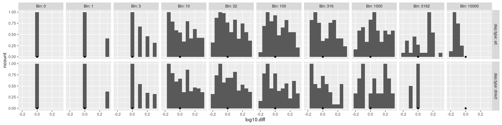
The histogram above shows the distribution of differences between the
actual number of reverse imports and the corresponding bin
center. Most of the differences fall between -0.2 and 0.2, which is to
be expected, since bin.dt used a bin size of 0.5 on the log scale.
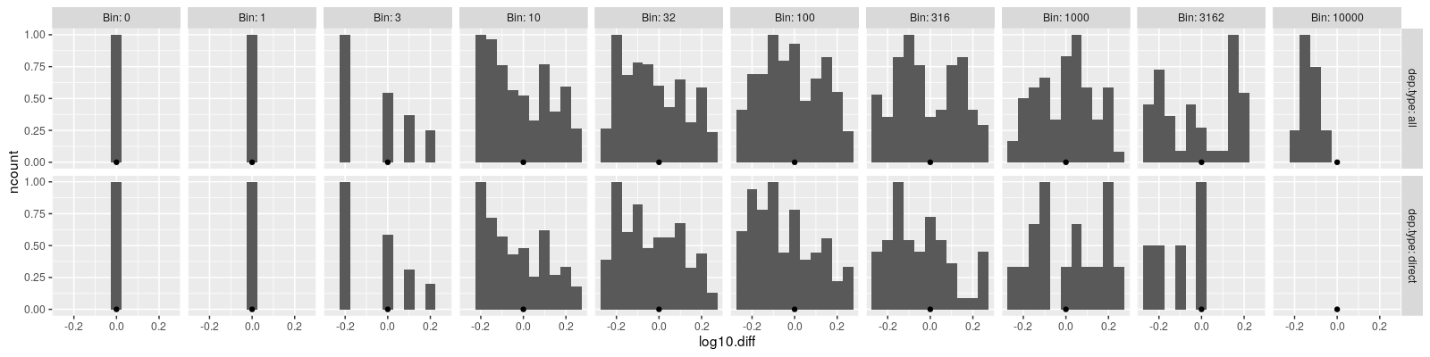
What if we did the same computation using the original distance scale?
bin.join <- bin.dt[dep.type.counts, .(
  dep.type, Package, Bin,
  log10.bin=x.log10.bin,
  rev.imports),
  roll="nearest",
  on=.(bin=rev.imports)
  ][, log10.rev.imports := log10(rev.imports)
  ][, log10.diff := ifelse(
    log10.rev.imports == -Inf, 0, log10.rev.imports-log10.bin)]
ggplot()+
  geom_histogram(aes(
    log10.diff, after_stat(ncount)),
    binwidth=bin.width,
    data=bin.join)+
  scale_x_continuous(breaks=seq(-1, 1, by=0.2))+
  geom_point(aes(x,y),data=data.table(x=0,y=0))+
  facet_grid(dep.type ~ Bin, labeller=label_both)
The bin assignments above were computed using a rolling join in the original reverse import count space (not the log space), so each histogram above is skewed to the right (the are more larger differences in each bin), as expected based on our theoretical analysis above which showed the asymmetric bins.
Finally we can compare the two histograms in the same plot. First we combine the two data sets created from rolling joins,
joinDT <- function(DT, distance, sign){
  DT[, .(distance, sign, log10.diff, dep.type, Bin)]
}
(bin.both.join <- rbind(
  joinDT(bin.join, "original", -1),
  joinDT(bin.log.join, "log", sign=1)))
##        distance  sign  log10.diff dep.type   Bin
##          <char> <num>       <num>   <char> <num>
##     1: original    -1 -0.06358680      all 10000
##     2: original    -1 -0.07216787      all 10000
##     3: original    -1 -0.07504911      all 10000
##     4: original    -1 -0.08223200      all 10000
##     5: original    -1 -0.09631327      all 10000
##    ---
## 75040:      log     1  0.00000000   direct     0
## 75041:      log     1  0.00000000   direct     0
## 75042:      log     1  0.00000000   direct     0
## 75043:      log     1  0.00000000   direct     0
## 75044:      log     1  0.00000000   direct     0
Then we compute histograms ourselves in the code below using the
hist function (instead of using geom_histogram as we did in the
code above),
max.abs.diff <- 0.4
breaks.vec <- seq(-max.abs.diff, max.abs.diff, by=bin.width)
(bin.both.hist <- bin.both.join[, {
  hlist <- hist(log10.diff, breaks.vec, plot=FALSE)
  with(hlist, data.table(log10.diff=mids, ncount=counts/max(counts)))
}, by=.(distance, sign, dep.type, Bin)])
##      distance  sign dep.type   Bin log10.diff ncount
##        <char> <num>   <char> <num>      <num>  <num>
##   1: original    -1      all 10000     -0.375      0
##   2: original    -1      all 10000     -0.325      0
##   3: original    -1      all 10000     -0.275      0
##   4: original    -1      all 10000     -0.225      0
##   5: original    -1      all 10000     -0.175      1
##  ---
## 604:      log     1   direct     0      0.175      0
## 605:      log     1   direct     0      0.225      0
## 606:      log     1   direct     0      0.275      0
## 607:      log     1   direct     0      0.325      0
## 608:      log     1   direct     0      0.375      0
The table above contains histograms of differences between actual
numbers of reverse imports, and the corresponding bin centers. The
ncount column is normalized between 0 and 1 so that the histograms
can be displayed on a common scale. In the code below we also compute
the mean of the differences, to see if there is any skew to larger
values than the bin center, as we would expect.
(bin.both.stats <- dcast(
  bin.both.join,
  distance + sign + dep.type + Bin ~ .,
  list(length, mean),
  value.var = "log10.diff"))
##     distance  sign dep.type   Bin log10.diff_length log10.diff_mean
##       <char> <num>   <char> <num>             <int>           <num>
##  1:      log     1      all     0             14290     0.000000000
##  2:      log     1      all     1              1572     0.000000000
##  3:      log     1      all     3              1394    -0.057402270
##  4:      log     1      all    10               673    -0.024827086
##  5:      log     1      all    32               379    -0.029358816
##  6:      log     1      all   100               211    -0.013584970
##  7:      log     1      all   316               111    -0.013580821
##  8:      log     1      all  1000                68    -0.004673764
##  9:      log     1      all  3162                45    -0.017145384
## 10:      log     1      all 10000                18    -0.132331020
## 11:      log     1   direct     0             14290     0.000000000
## 12:      log     1   direct     1              1876     0.000000000
## 13:      log     1   direct     3              1481    -0.066554348
## 14:      log     1   direct    10               642    -0.039676030
## 15:      log     1   direct    32               276    -0.038371816
## 16:      log     1   direct   100               117    -0.048097463
## 17:      log     1   direct   316                58    -0.042129331
## 18:      log     1   direct  1000                16     0.007191530
## 19:      log     1   direct  3162                 5    -0.102999626
## 20: original    -1      all     0             14290     0.000000000
## 21: original    -1      all     1              2217     0.087579769
## 22: original    -1      all     3               858     0.091649620
## 23: original    -1      all    10               625     0.039381623
## 24: original    -1      all    32               347     0.030125174
## 25: original    -1      all   100               197     0.038456067
## 26: original    -1      all   316               102     0.035174080
## 27: original    -1      all  1000                74     0.058778621
## 28: original    -1      all  3162                34     0.061689482
## 29: original    -1      all 10000                17    -0.128054947
## 30: original    -1   direct     0             14290     0.000000000
## 31: original    -1   direct     1              2581     0.082226326
## 32: original    -1   direct     3               908     0.086368755
## 33: original    -1   direct    10               562     0.032615799
## 34: original    -1   direct    32               249     0.031694090
## 35: original    -1   direct   100               103     0.028964698
## 36: original    -1   direct   316                48     0.004440089
## 37: original    -1   direct  1000                17     0.053739484
## 38: original    -1   direct  3162                 3    -0.027134169
##     distance  sign dep.type   Bin log10.diff_length log10.diff_mean
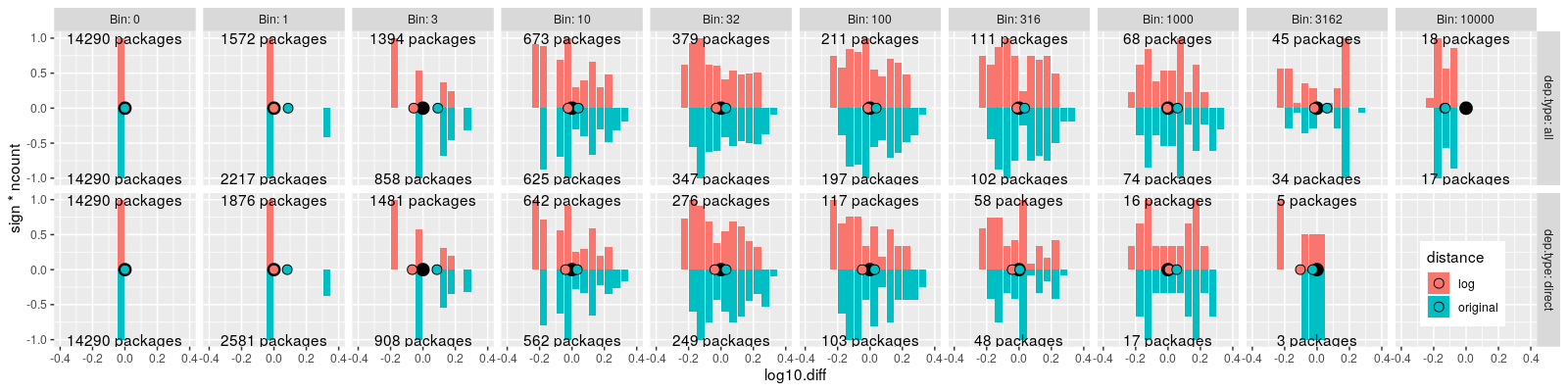
The table above has number of packages and mean difference columns, for every bin/histogram to plot, which we show below,
ggplot()+
  theme(legend.position=c(0.95, 0.2))+
  geom_bar(aes(
    log10.diff, sign*ncount, fill=distance),
    stat="identity",
    data=bin.both.hist)+
  geom_text(aes(
    0, sign, label=sprintf(
      "%d packages", log10.diff_length)),
    data=bin.both.stats)+
  geom_point(aes(
    x,y),
    size=4,
    data=data.table(x=0,y=0))+
  geom_point(aes(
    log10.diff_mean, 0, fill=distance),
    data=bin.both.stats,
    size=3,
    shape=21)+
  facet_grid(dep.type ~ Bin, labeller=label_both)