Learning with Area Under the Min
My collaborator Joe Barr of Acronis is working on an application of machine learning to predicting security vulnerabilities based on source code analysis, and a database of exploits. The data they are using for training/testing their models is highly imbalanced so I suggested trying my new Area Under the Min(FP,FN) loss function (AUM). After talking with them about the easiest way to try this new loss function on their data, I coded it in torch and verified that the gradients computed by torch are reasonable with respect to the expected directional directives. But does it work for learning? Yes, it does, as I show below.
Reading and scaling spam data
As an example data set, consider the spam data, one of the examples from the Elements of Statistical Learning textbook.
import pandas as pd
spam_df = pd.read_csv(
    "~/teaching/cs570-spring-2022/data/spam.data",
    header=None,
    sep=" ")
spam_df
##         0     1     2    3     4     5   ...     52     53     54   55    56  57
## 0     0.00  0.64  0.64  0.0  0.32  0.00  ...  0.000  0.000  3.756   61   278   1
## 1     0.21  0.28  0.50  0.0  0.14  0.28  ...  0.180  0.048  5.114  101  1028   1
## 2     0.06  0.00  0.71  0.0  1.23  0.19  ...  0.184  0.010  9.821  485  2259   1
## 3     0.00  0.00  0.00  0.0  0.63  0.00  ...  0.000  0.000  3.537   40   191   1
## 4     0.00  0.00  0.00  0.0  0.63  0.00  ...  0.000  0.000  3.537   40   191   1
## ...    ...   ...   ...  ...   ...   ...  ...    ...    ...    ...  ...   ...  ..
## 4596  0.31  0.00  0.62  0.0  0.00  0.31  ...  0.000  0.000  1.142    3    88   0
## 4597  0.00  0.00  0.00  0.0  0.00  0.00  ...  0.000  0.000  1.555    4    14   0
## 4598  0.30  0.00  0.30  0.0  0.00  0.00  ...  0.000  0.000  1.404    6   118   0
## 4599  0.96  0.00  0.00  0.0  0.32  0.00  ...  0.000  0.000  1.147    5    78   0
## 4600  0.00  0.00  0.65  0.0  0.00  0.00  ...  0.000  0.000  1.250    5    40   0
##
## [4601 rows x 58 columns]
After reading them into python above, we scale and center the inputs/features below,
import numpy as np
spam_features = spam_df.iloc[:,:-1].to_numpy()
spam_labels = spam_df.iloc[:,-1].to_numpy()
# 1. feature scaling
spam_mean = spam_features.mean(axis=0)
spam_sd = np.sqrt(spam_features.var(axis=0))
scaled_features = (spam_features-spam_mean)/spam_sd
scaled_features.mean(axis=0)
## array([ 1.85318688e-17,  2.77978032e-17,  2.47091584e-17,  0.00000000e+00,
##         4.94183168e-17,  3.70637376e-17, -2.47091584e-17,  0.00000000e+00,
##         2.47091584e-17,  1.23545792e-17, -2.47091584e-17,  6.94945080e-18,
##         0.00000000e+00, -3.39750928e-17,  0.00000000e+00,  7.41274751e-17,
##        -1.23545792e-17, -2.47091584e-17,  8.64820543e-17, -1.23545792e-17,
##        -4.94183168e-17, -1.85318688e-17,  0.00000000e+00, -2.47091584e-17,
##         0.00000000e+00,  1.23545792e-17, -1.23545792e-17,  0.00000000e+00,
##        -1.23545792e-17, -3.70637376e-17,  0.00000000e+00, -3.70637376e-17,
##         6.17728960e-18,  1.85318688e-17, -1.85318688e-17,  1.23545792e-17,
##        -3.70637376e-17,  0.00000000e+00,  0.00000000e+00,  2.47091584e-17,
##         0.00000000e+00, -5.55956064e-17, -4.32410272e-17,  1.85318688e-17,
##        -2.47091584e-17, -2.47091584e-17, -1.85318688e-17, -6.17728960e-18,
##         3.08864480e-17, -7.41274751e-17,  1.54432240e-17,  0.00000000e+00,
##        -2.47091584e-17,  0.00000000e+00,  4.32410272e-17,  1.23545792e-17,
##         2.47091584e-17])
scaled_features.var(axis=0)
## array([1., 1., 1., 1., 1., 1., 1., 1., 1., 1., 1., 1., 1., 1., 1., 1., 1.,
##        1., 1., 1., 1., 1., 1., 1., 1., 1., 1., 1., 1., 1., 1., 1., 1., 1.,
##        1., 1., 1., 1., 1., 1., 1., 1., 1., 1., 1., 1., 1., 1., 1., 1., 1.,
##        1., 1., 1., 1., 1., 1.])
scaled_features
## array([[-3.42433707e-01,  3.30884903e-01,  7.12858774e-01, ...,
##         -4.52472762e-02,  4.52979198e-02, -8.72413388e-03],
##        [ 3.45359395e-01,  5.19091945e-02,  4.35129540e-01, ...,
##         -2.44326749e-03,  2.50562832e-01,  1.22832407e+00],
##        [-1.45921392e-01, -1.65071912e-01,  8.51723390e-01, ...,
##          1.45920848e-01,  2.22110599e+00,  3.25873251e+00],
##        ...,
##        [ 6.40127868e-01, -1.65071912e-01,  3.83734930e-02, ...,
##         -1.19382054e-01, -2.36941335e-01, -2.72627750e-01],
##        [ 2.80176333e+00, -1.65071912e-01, -5.56760578e-01, ...,
##         -1.27482666e-01, -2.42072958e-01, -3.38603654e-01],
##        [-3.42433707e-01, -1.65071912e-01,  7.32696576e-01, ...,
##         -1.24236117e-01, -2.42072958e-01, -4.01280763e-01]])
The above output indicates that each feature column is indeed scaled to mean 0 and variance 1.
Dividing the data into subtrain and validation sets
Next, we randomly divide the data into a subtrain and validation set. The gradient descent parameter updates will be computed using the subtrain set, and the validation set will be used to check for overfitting.
np.random.seed(1)
n_folds = 5
fold_vec = np.random.randint(low=0, high=n_folds, size=spam_labels.size)
validation_fold = 0
is_set_dict = {
    "validation":fold_vec == validation_fold,
    "subtrain":fold_vec != validation_fold,
}
After having defined logical vectors above that indicate each set, we use them below to construct the corresponding tensors,
import torch
set_features = {}
set_labels = {}
for set_name, is_set in is_set_dict.items():
    set_features[set_name] = torch.from_numpy(
        scaled_features[is_set,:]).float()
    set_labels[set_name] = torch.from_numpy(
        spam_labels[is_set]).float()
{set_name:array.shape for set_name, array in set_features.items()}
## {'validation': torch.Size([921, 57]), 'subtrain': torch.Size([3680, 57])}
The output above shows the number of rows and columns in each data set.
Defining Dataset and DataLoader, neural network, loss function
To do the gradient descent learning randomly with a given batch size, it is easiest in torch to create a Dataset sub-class and a DataLoader instance, as we do below:
class CSV(torch.utils.data.Dataset):
    def __init__(self, features, labels):
        self.features = features
        self.labels = labels
    def __getitem__(self, item):
        return self.features[item,:], self.labels[item]
    def __len__(self):
        return len(self.labels)
subtrain_dataset = CSV(set_features["subtrain"], set_labels["subtrain"])
subtrain_dataloader = torch.utils.data.DataLoader(
    subtrain_dataset, batch_size=20, shuffle=True)
Next we define a neural network below with a single hidden layer of 200 hidden units,
nrow, ncol = set_features["subtrain"].shape
class NNet(torch.nn.Module):
    def __init__(self, n_hidden=200):
        super(NNet, self).__init__()
        self.seq = torch.nn.Sequential(
            torch.nn.Linear(ncol, n_hidden),
            torch.nn.ReLU(),
            torch.nn.Linear(n_hidden, 1)
            )
    def forward(self, feature_mat):
        return self.seq(feature_mat)
Below we define the AUM loss function and a helper function which we use to compute the loss during each gradient descent batch, and at the end of every epoch during the subtrain/validation loss computation,
def AUM(pred_tensor, label_tensor):
    """Area Under Min(FP,FN)

    Loss function for imbalanced binary classification
    problems. Minimizing AUM empirically results in maximizing Area
    Under the ROC Curve (AUC). Arguments: pred_tensor and label_tensor
    should both be 1d tensors (vectors of real-valued predictions and
    labels for each observation in the set/batch).

    """
    fn_diff = torch.where(label_tensor == 1, -1, 0)
    fp_diff = torch.where(label_tensor == 1, 0, 1)
    thresh_tensor = -pred_tensor.flatten()
    sorted_indices = torch.argsort(thresh_tensor)
    sorted_fp_cum = fp_diff[sorted_indices].cumsum(axis=0)
    sorted_fn_cum = -fn_diff[sorted_indices].flip(0).cumsum(axis=0).flip(0)
    sorted_thresh = thresh_tensor[sorted_indices]
    sorted_is_diff = sorted_thresh.diff() != 0
    sorted_fp_end = torch.cat([sorted_is_diff, torch.tensor([True])])
    sorted_fn_end = torch.cat([torch.tensor([True]), sorted_is_diff])
    uniq_thresh = sorted_thresh[sorted_fp_end]
    uniq_fp_after = sorted_fp_cum[sorted_fp_end]
    uniq_fn_before = sorted_fn_cum[sorted_fn_end]
    uniq_min = torch.minimum(uniq_fn_before[1:], uniq_fp_after[:-1])
    return torch.mean(uniq_min * uniq_thresh.diff())

def compute_loss_pred(features, labels):
    pred_mat = model(features)
    pred_vec = pred_mat.reshape(len(pred_mat))
    return AUM(pred_vec, labels), pred_vec

from pytorch_lightning.metrics.classification import AUROC
compute_auc = AUROC()
We additionally use AUROC to compute the Area Under the ROC Curve.
Learning iterations
Finally we use a for loop over epochs below to do the gradient descent learning. Note the step size of the Adam optimizer was chosen to be small enough such that the loss decreases smoothly (no abrupt jumps up), but big enough so that the loss is minimized within a reasonable number of epochs.
loss_df_list = []
max_epochs=100
torch.manual_seed(1)
## <torch._C.Generator object at 0x0000000060DDF490>
model = NNet()
optimizer = torch.optim.Adam(model.parameters(), lr=0.00004)
for epoch in range(max_epochs):
    # first update weights.
    for batch_features, batch_labels in subtrain_dataloader:
        optimizer.zero_grad()
        batch_loss, pred_vec = compute_loss_pred(batch_features, batch_labels)
        batch_loss.backward()
        optimizer.step()
    # then compute subtrain/validation loss.
    for set_name in set_features:
        feature_mat = set_features[set_name]
        label_vec = set_labels[set_name]
        set_loss, pred_vec = compute_loss_pred(feature_mat, label_vec)
        loss_df_list.append(pd.DataFrame({
            "epoch":[epoch],
            "set_name":[set_name],
            "variable":["AUM"],
            "value":set_loss.detach().numpy(),
            }))
        loss_df_list.append(pd.DataFrame({
            "epoch":[epoch],
            "set_name":[set_name],
            "variable":["AUC"],
            "value":compute_auc(pred_vec, label_vec).detach().numpy(),
            }))
loss_df = pd.concat(loss_df_list)
Finally we visualize the subtrain/validation loss and AUC using plotnine,
import plotnine as p9
gg = p9.ggplot()+\
    p9.facet_grid("variable ~ .", labeller="label_both", scales="free")+\
    p9.geom_line(
        p9.aes(
            x="epoch",
            y="value",
            color="set_name"
        ),
        data=loss_df)
show(gg, "AUM-AUC")
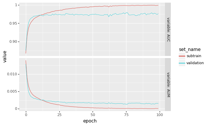
The plot above shows that the algorithm clearly is learning, and that decreasing the AUM results in increased AUC.