Update about data reshaping and visualization in R and python
R approach for histogram
My paper about regular expressions for data reshaping was recently accepted into R journal. I used visualization of the iris data as a example to motivate reshaping. Recall the iris data look like this,
head(iris)
##   Sepal.Length Sepal.Width Petal.Length Petal.Width Species
## 1          5.1         3.5          1.4         0.2  setosa
## 2          4.9         3.0          1.4         0.2  setosa
## 3          4.7         3.2          1.3         0.2  setosa
## 4          4.6         3.1          1.5         0.2  setosa
## 5          5.0         3.6          1.4         0.2  setosa
## 6          5.4         3.9          1.7         0.4  setosa
To make a facetted histogram, we need to combine the first four columns into a single column. To do that we define a regular expression to match those column names, then use that to reshape and visualize.
(iris.long <- nc::capture_melt_single(
  iris, part=".*", "[.]", dim=".*", value.name="cm"))
##        Species  part    dim  cm
##   1:    setosa Sepal Length 5.1
##   2:    setosa Sepal Length 4.9
##   3:    setosa Sepal Length 4.7
##   4:    setosa Sepal Length 4.6
##   5:    setosa Sepal Length 5.0
##  ---
## 596: virginica Petal  Width 2.3
## 597: virginica Petal  Width 1.9
## 598: virginica Petal  Width 2.0
## 599: virginica Petal  Width 2.3
## 600: virginica Petal  Width 1.8
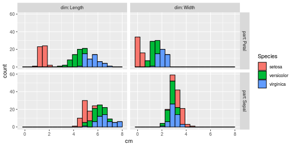
library(ggplot2)
## Keep up to date with changes at https://www.tidyverse.org/blog/
ggplot()+
  geom_histogram(aes(
    cm, fill=Species),
    color="black",
    bins=20,
    data=iris.long)+
  facet_grid(part ~ dim, labeller=label_both)
Recently data.table merged my PR which implements similar functionality:
library(data.table)
## data.table 1.14.1 IN DEVELOPMENT built 2021-05-25 12:11:15 UTC; tdhock using 1 threads (see ?getDTthreads). Latest news: r-datatable.com
one.iris <- data.table(iris[1,])
nc::capture_melt_single(one.iris, part=".*", "[.]", dim=".*")
##    Species  part    dim value
## 1:  setosa Sepal Length   5.1
## 2:  setosa Sepal  Width   3.5
## 3:  setosa Petal Length   1.4
## 4:  setosa Petal  Width   0.2
data.table::melt(
  one.iris, measure.vars=measure(part, dim, pattern="(.*)[.](.*)"))
##    Species  part    dim value
## 1:  setosa Sepal Length   5.1
## 2:  setosa Sepal  Width   3.5
## 3:  setosa Petal Length   1.4
## 4:  setosa Petal  Width   0.2
This functionality is also implemented in the tidyr package:
pattern <- "(.*)[.](.*)"
tidyr::pivot_longer(
  one.iris,
  cols=matches(pattern),
  names_to=c("part", "dim"),
  names_pattern=pattern)
## # A tibble: 4 x 4
##   Species part  dim    value
##   <fct>   <chr> <chr>  <dbl>
## 1 setosa  Sepal Length   5.1
## 2 setosa  Sepal Width    3.5
## 3 setosa  Petal Length   1.4
## 4 setosa  Petal Width    0.2
Note that in the tidyr version above the pattern needs to be
repeated in the cols and the names_pattern arguments.
Comparison with python approaches for histogram
I was curious to investigate the state of python modules for
performing the same computations. Is it as easy as in R? The intent of
the R code above is to use a regex pattern to specify: (1) the set of
columns to melt/reshape/unpivot, and (2) the data to capture in the
dim and part columns of the output. So my code below tries to
translate that idea into python.
If you are limited to using pandas, this is possible but not easy. My
first attempt at the data reshaping involved melt,
import pandas as pd
one_iris=pd.DataFrame({
    "Sepal.Length":[5.1],
    "Sepal.Width":[3.5],
    "Petal.Length":[1.4],
    "Petal.Width":[0.2],
    "Species":"setosa"})
pattern = "(?P<part>.*)[.](?P<dim>.*)"
col_extract = one_iris.columns.to_series().str.extract(pattern)
id_vars = [
    name for name,matched in
    zip(one_iris.columns, col_extract.iloc[:,0].notna())
    if not matched]
one_long = one_iris.melt(id_vars=id_vars)
pd.concat([one_long["variable"].str.extract(pattern), one_long], axis=1)
##     part     dim Species      variable  value
## 0  Sepal  Length  setosa  Sepal.Length    5.1
## 1  Sepal   Width  setosa   Sepal.Width    3.5
## 2  Petal  Length  setosa  Petal.Length    1.4
## 3  Petal   Width  setosa   Petal.Width    0.2
That was complicated! Luckily there is another function,
import janitor
import re
names_to = list(re.compile(pattern).groupindex.keys())
one_iris.pivot_longer(
    index="Species",
    names_pattern=pattern,
    names_to=names_to)
##   Species   part     dim  value
## 0  setosa  Sepal  Length    5.1
## 1  setosa  Sepal   Width    3.5
## 2  setosa  Petal  Length    1.4
## 3  setosa  Petal   Width    0.2
That was much easier! Note that the names and sub-patterns for each
capture group were defined together in the same regular expression
string literal, which was then compiled to get the group names to pass
as the names_to argument. Note that the python iris data has
slightly different column names (no dot),
iris_url = "https://raw.github.com/pandas-dev/pandas/master/pandas/tests/io/data/csv/iris.csv"
iris_wide = pd.read_csv(iris_url)
iris_wide
##      SepalLength  SepalWidth  PetalLength  PetalWidth            Name
## 0            5.1         3.5          1.4         0.2     Iris-setosa
## 1            4.9         3.0          1.4         0.2     Iris-setosa
## 2            4.7         3.2          1.3         0.2     Iris-setosa
## 3            4.6         3.1          1.5         0.2     Iris-setosa
## 4            5.0         3.6          1.4         0.2     Iris-setosa
## ..           ...         ...          ...         ...             ...
## 145          6.7         3.0          5.2         2.3  Iris-virginica
## 146          6.3         2.5          5.0         1.9  Iris-virginica
## 147          6.5         3.0          5.2         2.0  Iris-virginica
## 148          6.2         3.4          5.4         2.3  Iris-virginica
## 149          5.9         3.0          5.1         1.8  Iris-virginica
##
## [150 rows x 5 columns]
So we must repeat those steps with a different pattern,
pattern = "(?P<part>Sepal|Petal)(?P<dim>Length|Width)"
names_to = list(re.compile(pattern).groupindex.keys())
iris_long = iris_wide.pivot_longer(
    index="Name",
    names_pattern=pattern,
    names_to=names_to,
    values_to="cm")
iris_long
##                Name   part     dim   cm
## 0       Iris-setosa  Sepal  Length  5.1
## 1       Iris-setosa  Sepal  Length  4.9
## 2       Iris-setosa  Sepal  Length  4.7
## 3       Iris-setosa  Sepal  Length  4.6
## 4       Iris-setosa  Sepal  Length  5.0
## ..              ...    ...     ...  ...
## 595  Iris-virginica  Petal   Width  2.3
## 596  Iris-virginica  Petal   Width  1.9
## 597  Iris-virginica  Petal   Width  2.0
## 598  Iris-virginica  Petal   Width  2.3
## 599  Iris-virginica  Petal   Width  1.8
##
## [600 rows x 4 columns]
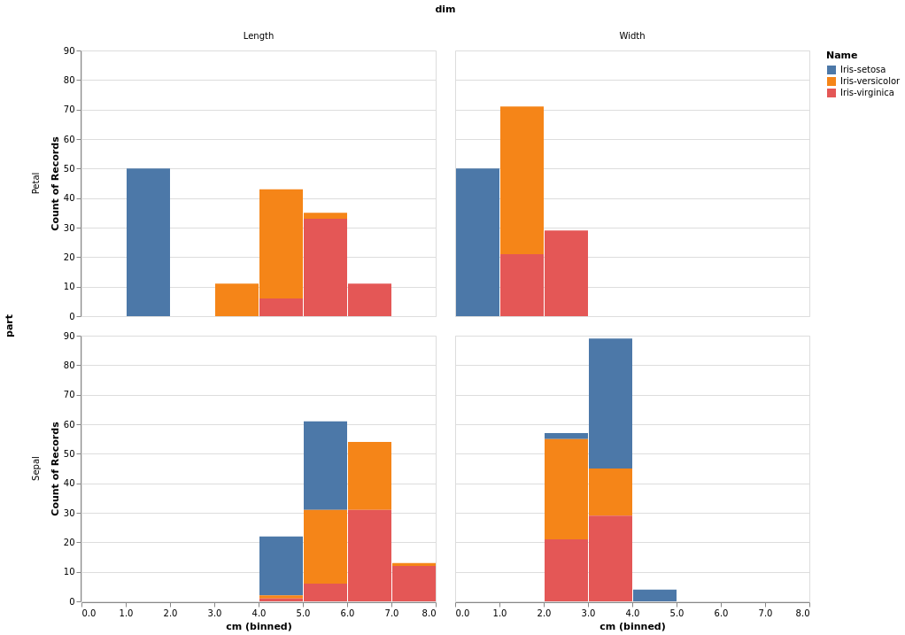
After that there are a number of modules to consider for making the
histogram. Again my goal is to replicate the intent of the R ggplot2
code, which says “each Species is a different color, and each part/dim
is a different panel.” At first I thought it may be possible to use
the default pandas plotting methods, but it is clear from the
docs
that there is no easy way to specify a variable to use for plotting in
different panels (a la facet_grid). Same for matplotlib and bokeh. A
python alternative is altair, which
does implement facets:
import altair as alt
chart = alt.Chart(iris_long).mark_bar().encode(
    alt.X("cm:Q", bin=True),
    y='count()',
    color="Name"
).facet(row="part", column="dim")
# need to do chart.show() then click save as PNG.
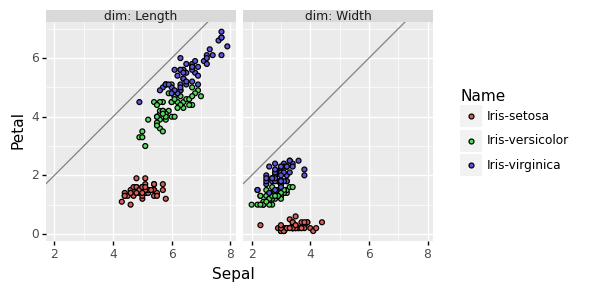
R approach for scatterplot comparing parts
Next plot from the paper was a facetted scatterplot comparing
parts… are Petals longer and/or wider than Sepals? To do that we
need to change the reshape operation so we output a Sepal and a
Petal column. In R this amounts to changing one of the regex group
names to a special value that is recognized as the keyword for
creating multiple output columns.
| Package | nc | data.table | tidyr |
| Function | capture_melt_multiple |
melt + measure |
pivot_longer |
| Keyword | column |
value.name |
.value |
nc::capture_melt_multiple(one.iris, column=".*", "[.]", dim=".*")
##    Species    dim Petal Sepal
## 1:  setosa Length   1.4   5.1
## 2:  setosa  Width   0.2   3.5
data.table::melt(
  one.iris, measure.vars=measure(value.name, dim, pattern="(.*)[.](.*)"))
##    Species    dim Sepal Petal
## 1:  setosa Length   5.1   1.4
## 2:  setosa  Width   3.5   0.2
pattern <- "(.*)[.](.*)"
tidyr::pivot_longer(
  one.iris,
  cols=matches(pattern),
  names_to=c(".value", "part"),
  names_pattern=pattern)
## # A tibble: 2 x 4
##   Species part   Sepal Petal
##   <fct>   <chr>  <dbl> <dbl>
## 1 setosa  Length   5.1   1.4
## 2 setosa  Width    3.5   0.2
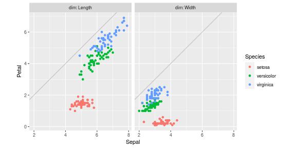
Doing that for the entire data set then plotting yields
(iris.parts <- nc::capture_melt_multiple(iris, column=".*", "[.]", dim=".*"))
##        Species    dim Petal Sepal
##   1:    setosa Length   1.4   5.1
##   2:    setosa Length   1.4   4.9
##   3:    setosa Length   1.3   4.7
##   4:    setosa Length   1.5   4.6
##   5:    setosa Length   1.4   5.0
##  ---
## 296: virginica  Width   2.3   3.0
## 297: virginica  Width   1.9   2.5
## 298: virginica  Width   2.0   3.0
## 299: virginica  Width   2.3   3.4
## 300: virginica  Width   1.8   3.0
ggplot()+
  coord_equal()+
  geom_abline(slope=1, intercept=0, color="grey")+
  geom_point(aes(
    Sepal, Petal, color=Species),
    data=iris.parts)+
  facet_grid(. ~ dim, labeller=label_both)
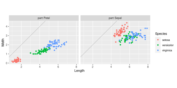
Python approach for scatterplot comparing parts
Python janitor can do the reshape (same .value keyword as in R to
indicate multiple outputs), but we can’t use a regex with named groups
this time, because the dot is not allowed:
re.compile("(?P<.value>Sepal|Petal)(?P<dim>Length|Width)")
## Error in py_call_impl(callable, dots$args, dots$keywords): error: bad character in group name '.value' at position 4
##
## Detailed traceback:
##   File "<string>", line 1, in <module>
##   File "/home/tdhock/.local/share/r-miniconda/envs/r-reticulate/lib/python3.6/re.py", line 233, in compile
##     return _compile(pattern, flags)
##   File "/home/tdhock/.local/share/r-miniconda/envs/r-reticulate/lib/python3.6/re.py", line 301, in _compile
##     p = sre_compile.compile(pattern, flags)
##   File "/home/tdhock/.local/share/r-miniconda/envs/r-reticulate/lib/python3.6/sre_compile.py", line 562, in compile
##     p = sre_parse.parse(p, flags)
##   File "/home/tdhock/.local/share/r-miniconda/envs/r-reticulate/lib/python3.6/sre_parse.py", line 855, in parse
##     p = _parse_sub(source, pattern, flags & SRE_FLAG_VERBOSE, 0)
##   File "/home/tdhock/.local/share/r-miniconda/envs/r-reticulate/lib/python3.6/sre_parse.py", line 416, in _parse_sub
##     not nested and not items))
##   File "/home/tdhock/.local/share/r-miniconda/envs/r-reticulate/lib/python3.6/sre_parse.py", line 647, in _parse
##     raise source.error(msg, len(name) + 1)
Well I guess you could use do the following,
names_pattern = "(?P<_value>Sepal|Petal)(?P<dim>Length|Width)"
names_to = [x.replace("_", ".") for x in re.compile(names_pattern).groupindex.keys()]
names_to
## ['.value', 'dim']
iris_parts = iris_wide.pivot_longer(
    index="Name",
    names_pattern=pattern,
    names_to=names_to)
iris_parts
##                Name     dim  Sepal  Petal
## 0       Iris-setosa  Length    5.1    1.4
## 1       Iris-setosa  Length    4.9    1.4
## 2       Iris-setosa  Length    4.7    1.3
## 3       Iris-setosa  Length    4.6    1.5
## 4       Iris-setosa  Length    5.0    1.4
## ..              ...     ...    ...    ...
## 295  Iris-virginica   Width    3.0    2.3
## 296  Iris-virginica   Width    2.5    1.9
## 297  Iris-virginica   Width    3.0    2.0
## 298  Iris-virginica   Width    3.4    2.3
## 299  Iris-virginica   Width    3.0    1.8
##
## [300 rows x 4 columns]
Now let’s try to plot with altair again,
import altair as alt
chart = alt.Chart(iris_parts).mark_circle().encode(
    x="Sepal",
    y="Petal",
    color="Name"
).facet(column="dim")
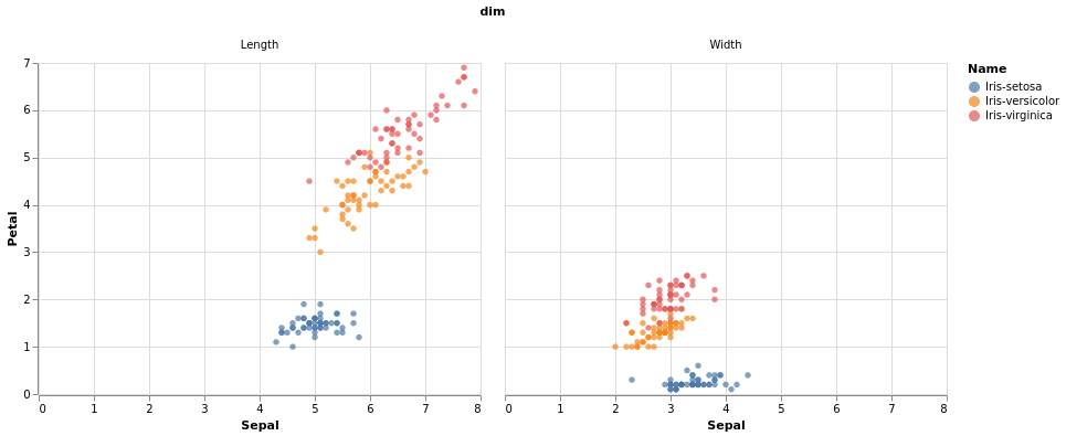
Two ggplot2 features which are missing in the altair plot above are
coord_equal and
geom_abline. These
are useful when you want to emphasize that the x and y axes have the
same units, so you can see if the data are above the
diagonal, are Petals longer/wider than Sepals?
So did you read my blog tutorial from last year, in which we explored python datatable and plotnine? Well, datatable still has not implemented the reshape/melt functionality, and plotnine still seems to have the best ggplot2 emulation:
import plotnine as p9
gg_scatter_parts = p9.ggplot()+\
    p9.geom_abline(
        slope=1, intercept=0,
        color="grey")+\
    p9.geom_point(
        p9.aes(x="Sepal", y="Petal", fill="Name"),
        iris_parts)+\
    p9.facet_grid(". ~ dim", labeller="label_both")+\
    p9.coord_equal()
So janitor + plotnine works well here! Incidentally, we can also do this reshape with plain pandas:
iris_wide["id"] = iris_wide.index
pd.wide_to_long(
    iris_wide, ["Petal", "Sepal"],
    i="id", j="dim", sep="", suffix="(Width|Length)"
).reset_index()
##       id     dim            Name  Petal  Sepal
## 0      0  Length     Iris-setosa    1.4    5.1
## 1      1  Length     Iris-setosa    1.4    4.9
## 2      2  Length     Iris-setosa    1.3    4.7
## 3      3  Length     Iris-setosa    1.5    4.6
## 4      4  Length     Iris-setosa    1.4    5.0
## ..   ...     ...             ...    ...    ...
## 295  145   Width  Iris-virginica    2.3    3.0
## 296  146   Width  Iris-virginica    1.9    2.5
## 297  147   Width  Iris-virginica    2.0    3.0
## 298  148   Width  Iris-virginica    2.3    3.4
## 299  149   Width  Iris-virginica    1.8    3.0
##
## [300 rows x 5 columns]
So pd.wide_to_long in python is similar to stats::reshape in R, in
that (1) two groups are assumed, and (2) it is assumed the .value /
value.name / column group comes first. In other words, these work
for this reshape operation, but they do NOT work for the similar
reshape in the next section (without some pre-processing of column
names).
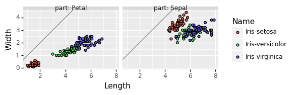
R approach for scatterplot comparing dims
In this section we reshape into Length and Width columns. In R we
just have to move the keyword from the first to the second group,
nc::capture_melt_multiple(one.iris, part=".*", "[.]", column=".*")
##    Species  part Length Width
## 1:  setosa Petal    1.4   0.2
## 2:  setosa Sepal    5.1   3.5
data.table::melt(
  one.iris, measure.vars=measure(part, value.name, pattern="(.*)[.](.*)"))
##    Species  part Length Width
## 1:  setosa Sepal    5.1   3.5
## 2:  setosa Petal    1.4   0.2
pattern <- "(.*)[.](.*)"
tidyr::pivot_longer(
  one.iris,
  cols=matches(pattern),
  names_to=c("part", ".value"),
  names_pattern=pattern)
## # A tibble: 2 x 4
##   Species part  Length Width
##   <fct>   <chr>  <dbl> <dbl>
## 1 setosa  Sepal    5.1   3.5
## 2 setosa  Petal    1.4   0.2
Doing that for the entire data set then plotting yields
(iris.dims <- nc::capture_melt_multiple(iris, part=".*", "[.]", column=".*"))
##        Species  part Length Width
##   1:    setosa Petal    1.4   0.2
##   2:    setosa Petal    1.4   0.2
##   3:    setosa Petal    1.3   0.2
##   4:    setosa Petal    1.5   0.2
##   5:    setosa Petal    1.4   0.2
##  ---
## 296: virginica Sepal    6.7   3.0
## 297: virginica Sepal    6.3   2.5
## 298: virginica Sepal    6.5   3.0
## 299: virginica Sepal    6.2   3.4
## 300: virginica Sepal    5.9   3.0
ggplot()+
  coord_equal()+
  geom_abline(slope=1, intercept=0, color="grey")+
  geom_point(aes(
    Length, Width, color=Species),
    data=iris.dims)+
  facet_grid(. ~ part, labeller=label_both)
Python approach for scatterplot comparing dims
As in the previous problem, we can use janitor + plotnine:
names_pattern = "(?P<part>Sepal|Petal)(?P<_value>Length|Width)"
names_to = [x.replace("_", ".") for x in re.compile(names_pattern).groupindex.keys()]
names_to
## ['part', '.value']
iris_dims = iris_wide.pivot_longer(
    index="Name",
    names_pattern=pattern,
    names_to=names_to)
## /home/tdhock/.local/share/r-miniconda/envs/r-reticulate/lib/python3.6/site-packages/janitor/utils.py:1500: FutureWarning: This dataframe has a column name that matches the 'value_name' column name of the resultiing Dataframe. In the future this will raise an error, please set the 'value_name' parameter of DataFrame.melt to a unique name.
iris_dims
##                Name   part  Length  Width   0
## 0       Iris-setosa  Petal     1.4    0.2 NaN
## 1       Iris-setosa  Petal     1.4    0.2 NaN
## 2       Iris-setosa  Petal     1.3    0.2 NaN
## 3       Iris-setosa  Petal     1.5    0.2 NaN
## 4       Iris-setosa  Petal     1.4    0.2 NaN
## ..              ...    ...     ...    ...  ..
## 295  Iris-virginica  Sepal     6.7    3.0 NaN
## 296  Iris-virginica  Sepal     6.3    2.5 NaN
## 297  Iris-virginica  Sepal     6.5    3.0 NaN
## 298  Iris-virginica  Sepal     6.2    3.4 NaN
## 299  Iris-virginica  Sepal     5.9    3.0 NaN
##
## [300 rows x 5 columns]
gg_scatter_dims = p9.ggplot()+\
    p9.geom_abline(
        slope=1, intercept=0,
        color="grey")+\
    p9.geom_point(
        p9.aes(x="Length", y="Width", fill="Name"),
        iris_dims)+\
    p9.facet_grid(". ~ part", labeller="label_both")+\
    p9.coord_equal()
No integrated type conversion in python
In R we can do type conversion during the reshape,
DT <- data.table(id=1, child1_sex="M", child1_age=34, child2_sex="F")
pattern <- "(.)_(.*)"
names_transform <- list(number_int=as.integer, .value=identity)
tidyr::pivot_longer(
  DT, matches(pattern),
  names_to=names(names_transform),
  names_transform=names_transform,
  names_pattern=pattern)
## # A tibble: 2 x 4
##      id number_int sex     age
##   <dbl>      <int> <chr> <dbl>
## 1     1          1 M        34
## 2     1          2 F        NA
print(
  melt(DT, measure.vars=measurev(
    names_transform, pattern=pattern, multiple.keyword=".value"))
, class=TRUE)
##       id number_int    sex   age
##    <num>      <int> <char> <num>
## 1:     1          1      M    34
## 2:     1          2      F    NA
number_pattern <- list(number_int=".", as.integer)
print(
  nc::capture_melt_multiple(
    DT, number_pattern, "_", column=".*", fill=TRUE)
, class=TRUE)
##       id number_int   age    sex
##    <num>      <int> <num> <char>
## 1:     1          1    34      M
## 2:     1          2    NA      F
Note that tidyr and data.table syntax require definition of the
regex pattern in a separately from the names/conversions which are
defined in names_transform. In contrast, the nc syntax allows
definition of these three related pieces of information together in
group-specific sub-pattern list variables, for example
number_pattern. The results above show that number_int is indeed
of type int — is this possible in python?
DT = pd.DataFrame({
    "id":[1],
    "child1_sex":["M"],
    "child1_age":[34],
    "child2_sex":["F"]
})
DT_long = DT.pivot_longer(
    index="id",
    names_pattern="(.)_(.*)",
    names_to = ["number", ".value"])
DT_long
##    id number sex   age
## 0   1      1   M  34.0
## 1   1      2   F   NaN
type(DT_long["number"][0])
## <class 'str'>
There is no names_transform argument in python (number is actually a
string), but you can always do the transform after the fact (less
efficient/convenient),
DT_long["number_int"] = DT_long["number"].astype(int)
DT_long
##    id number sex   age  number_int
## 0   1      1   M  34.0           1
## 1   1      2   F   NaN           2
type(DT_long["number_int"][0])
## <class 'numpy.int64'>
Conclusions
So in conclusion the python pivot_longer is a decent data reshaping
tool, but still is not quite as fully featured as the software we have
in R. In particular we observed the following:
- Named capture groups are supported in python, and are useful since they allow defining the capture group names and sub-patterns together in the regex string literal. This is an advantage over R tidyr, which does not support named groups because it uses the ICU C regex library (does not export of group names to R). Even better (in terms of keeping related information together) is the R nc syntax, which allows defining a list for each capture group that contains: (1) group name, (2) regex pattern, and (3) type conversion function.
- Named capture groups can not be easily used with python
pivot_longerfor reshape to multiple output columns. This is becausepivot_longeroutputs multiple value columns whennames_to=".value"is specified, but.valuecan not be used as a capture group name in the regex. We showed a workaround using the regex capture group named_valueand renamed to.value. - R packages provide integrated type conversion, but python
pivot_longerdoes not (although types can be converted after the reshape operation).
Of the python modules for visualization,
- neither bokeh, nor the pandas plot method, nor matplotlib, supports facets (subplots defined via column names).
- altair supports facets but does not support
coord_equalandgeom_abline. - plotnine seems to be the best way in python to emulate the functionality we have in R with ggplot2.