Computing K-means train/validation error
Today in my CS499/599 class on Unsupervised
Learning I explained
how to efficiently compute the train/validation error of the K-means
clustering algorithm in R. I only had time in class to explain a
method using array, but here I explain a few different methods.
Let’s use the classic iris data as a simple example. We begin by splitting the data into half train, half validation:
> X.mat <- as.matrix(iris[, 1:4])
> set.seed(1)
> shuffled.sets <- sample(rep(c("train", "validation"), l=nrow(X.mat)))
> table(shuffled.sets, iris$Species)

shuffled.sets setosa versicolor virginica
   train          22         31        22
   validation     28         19        28
Then we use the K-means algorithm to compute two cluster centers using only the train set:
> n.clusters <- 2
> kmeans.result <- stats::kmeans(X.mat[shuffled.sets=="train", ], n.clusters)
> kmeans.result$centers
  Sepal.Length Sepal.Width Petal.Length Petal.Width
1     6.280769    2.909615     4.892308   1.6576923
2     5.034783    3.404348     1.500000   0.2608696
The goal is to compute the total sum of squares for each set (train/validation). To do that we need to compute the sum of squares between each observation and each cluster center, then for each observation take the minimum over clusters. How to do that efficiently?
Multi-dimensional arrays
Multi-dimensional arrays can be used for fast vector operations in R. In this case we want an array with one element for each observation/feature/cluster combination, so we will use those names for the dimnames of our array:
> array.dim <- c(nrow(X.mat), ncol(X.mat), nrow(kmeans.result$centers))
> array.names <- list(obs=NULL, feature=NULL, cluster=NULL)
> X.array <- array(
+   X.mat, array.dim, array.names)
> head(X.array)
, , 1

      feature
obs    [,1] [,2] [,3] [,4]
  [1,]  5.1  3.5  1.4  0.2
  [2,]  4.9  3.0  1.4  0.2
  [3,]  4.7  3.2  1.3  0.2
  [4,]  4.6  3.1  1.5  0.2
  [5,]  5.0  3.6  1.4  0.2
  [6,]  5.4  3.9  1.7  0.4

, , 2

      feature
obs    [,1] [,2] [,3] [,4]
  [1,]  5.1  3.5  1.4  0.2
  [2,]  4.9  3.0  1.4  0.2
  [3,]  4.7  3.2  1.3  0.2
  [4,]  4.6  3.1  1.5  0.2
  [5,]  5.0  3.6  1.4  0.2
  [6,]  5.4  3.9  1.7  0.4

> head(X.mat)
     Sepal.Length Sepal.Width Petal.Length Petal.Width
[1,]          5.1         3.5          1.4         0.2
[2,]          4.9         3.0          1.4         0.2
[3,]          4.7         3.2          1.3         0.2
[4,]          4.6         3.1          1.5         0.2
[5,]          5.0         3.6          1.4         0.2
[6,]          5.4         3.9          1.7         0.4
Note how the third dimension has two elements, each a copy of the iris data matrix (one copy for each cluster center). We also need an array with copies of the cluster centers:
> m.array <- array(
+   rep(t(kmeans.result$centers), each=nrow(X.mat)), array.dim, array.names)
> head(m.array)
, , 1

      feature
obs        [,1]     [,2]     [,3]     [,4]
  [1,] 6.280769 2.909615 4.892308 1.657692
  [2,] 6.280769 2.909615 4.892308 1.657692
  [3,] 6.280769 2.909615 4.892308 1.657692
  [4,] 6.280769 2.909615 4.892308 1.657692
  [5,] 6.280769 2.909615 4.892308 1.657692
  [6,] 6.280769 2.909615 4.892308 1.657692

, , 2

      feature
obs        [,1]     [,2] [,3]      [,4]
  [1,] 5.034783 3.404348  1.5 0.2608696
  [2,] 5.034783 3.404348  1.5 0.2608696
  [3,] 5.034783 3.404348  1.5 0.2608696
  [4,] 5.034783 3.404348  1.5 0.2608696
  [5,] 5.034783 3.404348  1.5 0.2608696
  [6,] 5.034783 3.404348  1.5 0.2608696

> kmeans.result$centers
  Sepal.Length Sepal.Width Petal.Length Petal.Width
1     6.280769    2.909615     4.892308   1.6576923
2     5.034783    3.404348     1.500000   0.2608696
Note how we used rep and t on the cluster center matrix to
broadcast the values in the correct order. The computation then uses
array-array arithmetic and apply functions:
> squares.array <- (X.array-m.array)^2
> sum.squares.mat <- apply(squares.array, c("obs", "cluster"), sum)
> min.vec <- apply(sum.squares.mat, "obs", min)
> tapply(min.vec, shuffled.sets, sum)
     train validation
  78.48633   74.84365
> kmeans.result$tot.withinss
[1] 78.48633
Note that our computation agrees with the result from kmeans.
Analogous method using data.table
The previous method involves computing/storing an array with one element for every observation/feature/cluster combination. How would we do an analogous computation using data.table? First we convert the matrices of data and cluster centers into data tables:
> (X.dt <- data.table::data.table(
+   value=as.numeric(X.mat),
+   obs=as.integer(row(X.mat)),
+   feature=as.integer(col(X.mat))))
     value obs feature
  1:   5.1   1       1
  2:   4.9   2       1
  3:   4.7   3       1
  4:   4.6   4       1
  5:   5.0   5       1
 ---
596:   2.3 146       4
597:   1.9 147       4
598:   2.0 148       4
599:   2.3 149       4
600:   1.8 150       4
> (m.dt <- data.table::data.table(
+   center=as.numeric(kmeans.result$centers),
+   cluster=as.integer(row(kmeans.result$centers)),
+   feature=as.integer(col(kmeans.result$centers))))
      center cluster feature
1: 6.2807692       1       1
2: 5.0347826       2       1
3: 2.9096154       1       2
4: 3.4043478       2       2
5: 4.8923077       1       3
6: 1.5000000       2       3
7: 1.6576923       1       4
8: 0.2608696       2       4
Then we do a cartesian join on feature between these two data tables, in order to consider all possible combinations of observation/feature/cluster:
> squares.dt <- X.dt[m.dt, on="feature", allow.cartesian=TRUE]
> squares.dt[, square := (value-center)^2 ]
> squares.dt
      value obs feature    center cluster   square
   1:   5.1   1       1 6.2807692       1 1.394216
   2:   4.9   2       1 6.2807692       1 1.906524
   3:   4.7   3       1 6.2807692       1 2.498831
   4:   4.6   4       1 6.2807692       1 2.824985
   5:   5.0   5       1 6.2807692       1 1.640370
  ---
1196:   2.3 146       4 0.2608696       2 4.158053
1197:   1.9 147       4 0.2608696       2 2.686749
1198:   2.0 148       4 0.2608696       2 3.024575
1199:   2.3 149       4 0.2608696       2 4.158053
1200:   1.8 150       4 0.2608696       2 2.368922
> length(squares.array)
[1] 1200
Note that the code above shows that the storage complexity is the same
as in the previous array method (1200 is the number of combinations of
observation/feature/cluster). The final step is to use data table
summarization oprations using by (analogous to the apply operations
in the previous method):
> sum.squares.dt <- squares.dt[, .(
+   sum.squares=sum(square)
+ ), by=c("obs", "cluster")]
> min.dt <- sum.squares.dt[, .(
+   min.ss=min(sum.squares)
+ ), by="obs"]
> min.dt[, .(
+   tot.withinss=sum(min.ss)
+ ), by=.(set=shuffled.sets[obs])]
          set tot.withinss
1: validation     74.84365
2:      train     78.48633
> kmeans.result$tot.withinss
[1] 78.48633
Again the resulting train sum of squares is consistent with the value returned by the kmeans function.
More efficient method using data table
Both methods above require memory storage which is proportional to the number of combinations of observation/feature/cluster, which may be prohibitive for big data sets. How can we do the same computation but using less memory storage?
We can use data.table, but in a different way. Rather than beginning with a cartesian join (which requires a lot of memory), we instead create a data table with columns for set and observation id:
> (set.obs.ids <- data.table::data.table(
+   set=shuffled.sets, obs=seq_along(shuffled.sets)))
            set obs
  1: validation   1
  2:      train   2
  3: validation   3
  4: validation   4
  5: validation   5
 ---
146: validation 146
147:      train 147
148: validation 148
149: validation 149
150: validation 150
Then we need to think about the return value that we want, which is a
data table with two rows (one for each set) and two columns (set,
tot.withinss). To get that data table we use two nested data table
summarization operations: the outer one by=set and the inner one
by=obs:
> set.obs.ids[, {
+   set.obs.mins <- .SD[, {
+     diff.mat <- X.mat[obs, ] - t(kmeans.result$centers)
+     .(min.ss=min(colSums(diff.mat^2)))
+   }, by="obs"]
+   set.obs.mins[, .(tot.withinss=sum(min.ss))]
+ }, by="set"]
          set tot.withinss
1: validation     74.84365
2:      train     78.48633
> kmeans.result$tot.withinss
[1] 78.48633
The code above uses .SD which means the Subset of Data corresponding
to a single value of by=set. Using .SD[, .(min.ss=...), by=obs]
means to compute, for each observation in that set, the minimum sum of
squares across all clusters.
Analogous version using for loops
The data table code above may seem a bit strange, but it is really
just using by instead of for loops. Here is a translation which is
perhaps easier for some readers to understand:
> tot.withinss <- structure(
+   rep(NA_real_, length(set.prop.vec)),
+   names=names(set.prop.vec))
> for(set in names(set.prop.vec)){
+   X.set <- X.mat[shuffled.sets == set, ]
+   set.obs.mins <- rep(NA_real_, nrow(X.set))
+   for(obs in 1:nrow(X.set)){
+     diff.mat <- X.set[obs, ] - t(kmeans.result$centers)
+     set.obs.mins[[obs]] <- min(colSums(diff.mat^2))
+   }
+   tot.withinss[[set]] <- sum(set.obs.mins)
+ }
> tot.withinss
validation      train
  74.84365   78.48633
> kmeans.result$tot.withinss
[1] 78.48633
In the code above X.set is the analog of .SD (the data for one
set), and in each iteration of the for loops we fill in an entry of
the numeric vectors set.obs.mins and then tot.withinss.
List of data tables idiom
Yet another method is to use the list of data tables idiom,
> for(set in names(set.prop.vec)){
+   X.set <- X.mat[shuffled.sets == set, ]
+   set.obs.mins.dt.list <- list()
+   for(obs in 1:nrow(X.set)){
+     diff.mat <- X.set[obs, ] - t(kmeans.result$centers)
+     set.obs.mins.dt.list[[obs]] <- data.table::data.table(
+       obs, min.ss=min(colSums(diff.mat^2)))
+   }
+   set.obs.mins.dt <- do.call(rbind, set.obs.mins.dt.list)
+   tot.withinss.dt.list[[set]] <- set.obs.mins.dt[, .(
+     set,
+     tot.withinss=sum(min.ss))]
+ }
> (tot.withinss.dt <- do.call(rbind, tot.withinss.dt.list))
          set tot.withinss
1: validation     74.84365
2:      train     78.48633
> kmeans.result$tot.withinss
[1] 78.48633
Other methods
There are three different methods we have seen above:
- for loop using base R data structures, fill an entry of the matrix during each iteration.
- for loop using list of data tables idiom.
- data table summarization using
byinstead of a for loop.
There are also three different things we can do the loop/by over:
- observations only.
- clusters only.
- sets and observations.
Exercise for the reader: implement all 9 combinations of the above.
Comparing computational requirements
The methods presented above all compute the same result, but which is most efficient?
The figure below presents a comparison of timings of several different methods, for the zip.test data set (7291 x 256) and from 2 to 5 clusters.
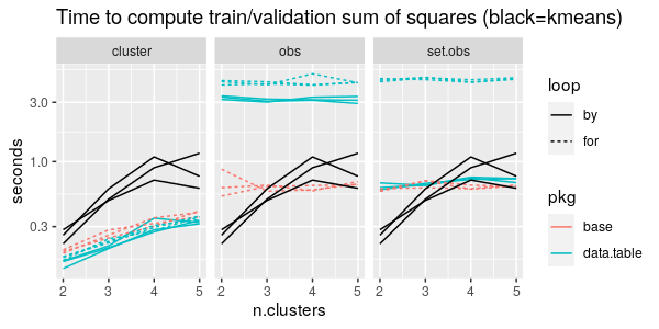
From the first panel above we can see that all three pkg/loop combinations take about the same time, less than kmeans itself (black), if we do by/for over clusters only.
From the second panel above we can see that data.table methods are actually much slower than the base R for loop, when we are doing by/for over observations only.
From the third panel above we can see that if we do by/for over both set and observations, then the list of data tables idiom is much slower than the other two methods (data.table by and base R for loop).
Overall from the figure above it is clear that the most important thing to consider in implementing this computation is to minimize the number of things to iterate over (the number of clusters is definitely smaller than the number of observations).
The figure below takes the best method from above and compares it to the all.combos (array/cartesian join) methods:
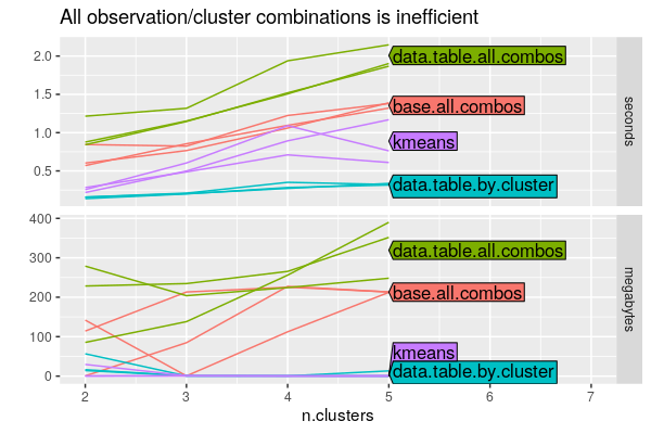
The top panel shows that the all.combos methods take more time than
the data.table.by.cluster method (which was tied as fastest in the
previous figure).
It is clear from the bottom panel that the all.combos methods take
much more memory, which is expected.
Overall it is clear that the cartesian join should be avoided if at all possible, and when writing by/for operations you should minimize the number of items you iterate over.