Positioning Method for 2 groups of longitudinal data. One curve
is on top of the other one (on average), so we label the top one
at its maximal point, and the bottom one at its minimal
point. Vertical justification is chosen to minimize collisions
with the other line. This may not work so well for data with high
variability, but then again lineplots may not be the best for
these data either.
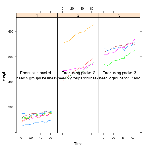 |
bodyweight
data(BodyWeight,package="nlme")
library(lattice)
p <- xyplot(weight~Time|Diet,BodyWeight,groups=Rat,type='l',
       layout=c(3,1),xlim=c(-10,75))
direct.label(p,"lines2")
|
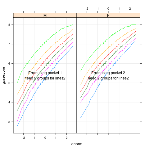 |
chemqqmathscore
data(Chem97,package="mlmRev")
library(lattice)
p <- qqmath(~gcsescore|gender,Chem97,groups=factor(score),
       type=c('l','g'),f.value=ppoints(100))
direct.label(p,"lines2")
|
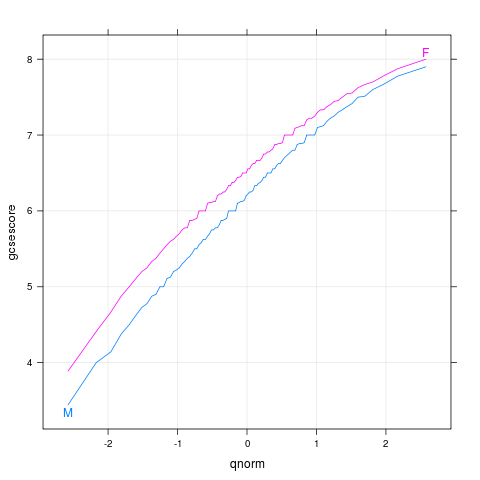 |
chemqqmathsex
data(Chem97,package="mlmRev")
library(lattice)
p <- qqmath(~gcsescore,Chem97,groups=gender,
       type=c("l","g"),f.value=ppoints(100))
direct.label(p,"lines2")
|
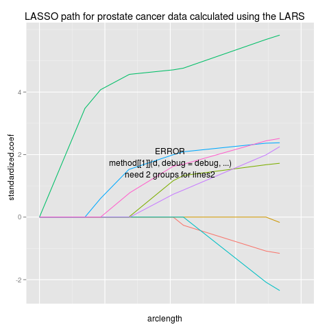 |
lars
data(prostate,package="ElemStatLearn")
pros <- subset(prostate,select=-train,train==TRUE)
ycol <- which(names(pros)=="lpsa")
x <- as.matrix(pros[-ycol])
y <- pros[[ycol]]
library(lars)
fit <- lars(x,y,type="lasso")
beta <- scale(coef(fit),FALSE,1/fit$normx)
arclength <- rowSums(abs(beta))
library(reshape2)
path <- data.frame(melt(beta),arclength)
names(path)[1:3] <- c("step","variable","standardized.coef")
library(ggplot2)
p <- ggplot(path,aes(arclength,standardized.coef,colour=variable))+
  geom_line(aes(group=variable))+
  ggtitle("LASSO path for prostate cancer data calculated using the LARS")+
  xlim(0,20)
direct.label(p,"lines2")
|
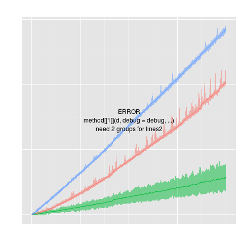 |
projectionSeconds
data(projectionSeconds, package="directlabels")
p <- ggplot(projectionSeconds, aes(vector.length/1e6))+
  geom_ribbon(aes(ymin=min, ymax=max,
                  fill=method, group=method), alpha=1/2)+
  geom_line(aes(y=mean, group=method, colour=method))+
  ggtitle("Projection Time against Vector Length (Sparsity = 10%)")+
  guides(fill="none")+
  ylab("Runtime (s)")
direct.label(p,"lines2")
|
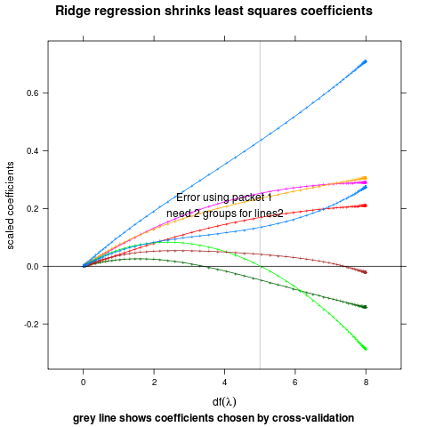 |
ridge
## complicated ridge regression lineplot ex. fig 3.8 from Elements of
## Statistical Learning, Hastie et al.
myridge <- function(f,data,lambda=c(exp(-seq(-15,15,l=200)),0)){
  require(MASS)
  require(reshape2)
  fit <- lm.ridge(f,data,lambda=lambda)
  X <- data[-which(names(data)==as.character(f[[2]]))]
  Xs <- svd(scale(X)) ## my d's should come from the scaled matrix
  dsq <- Xs$d^2
  ## make the x axis degrees of freedom
  df <- sapply(lambda,function(l)sum(dsq/(dsq+l)))
  D <- data.frame(t(fit$coef),lambda,df) # scaled coefs
  molt <- melt(D,id=c("lambda","df"))
  ## add in the points for df=0
  limpts <- transform(subset(molt,lambda==0),lambda=Inf,df=0,value=0)
  rbind(limpts,molt)
}
data(prostate,package="ElemStatLearn")
pros <- subset(prostate,train==TRUE,select=-train)
m <- myridge(lpsa~.,pros)
library(lattice)
p <- xyplot(value~df,m,groups=variable,type="o",pch="+",
       panel=function(...){
         panel.xyplot(...)
         panel.abline(h=0)
         panel.abline(v=5,col="grey")
       },
       xlim=c(-1,9),
       main="Ridge regression shrinks least squares coefficients",
       ylab="scaled coefficients",
       sub="grey line shows coefficients chosen by cross-validation",
       xlab=expression(df(lambda)))
direct.label(p,"lines2")
|
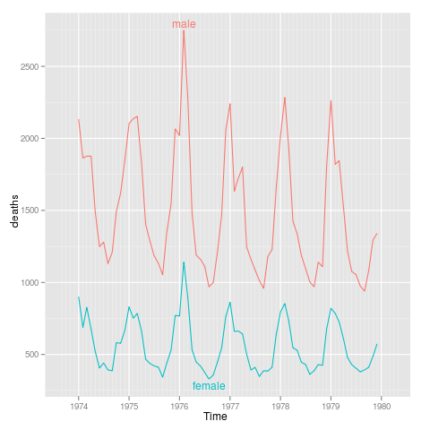 |
sexdeaths
library(ggplot2)
tx <- time(mdeaths)
Time <- ISOdate(floor(tx),round(tx%%1 * 12)+1,1,0,0,0)
uk.lung <- rbind(data.frame(Time,sex="male",deaths=as.integer(mdeaths)),
                 data.frame(Time,sex="female",deaths=as.integer(fdeaths)))
p <- qplot(Time,deaths,data=uk.lung,colour=sex,geom="line")+
  xlim(ISOdate(1973,9,1),ISOdate(1980,4,1))
direct.label(p,"lines2")
|